Overfitting and Regularization

A model that memorises its training set — including its noise and its idiosyncrasies — is worthless the moment it sees a new example. Regularisation is the collection of techniques that stop a model from doing that, by encoding a preference for simpler explanations somewhere in the loss, the data, or the training procedure itself.

Key idea

Every regulariser encodes a preference for simpler explanations, whether through the loss, the data, or the training procedure.

Overfitting is visible as a gap that opens between the two curves. The validation minimum is the early-stopping point; everything to the right of it buys training loss at the cost of generalisation.

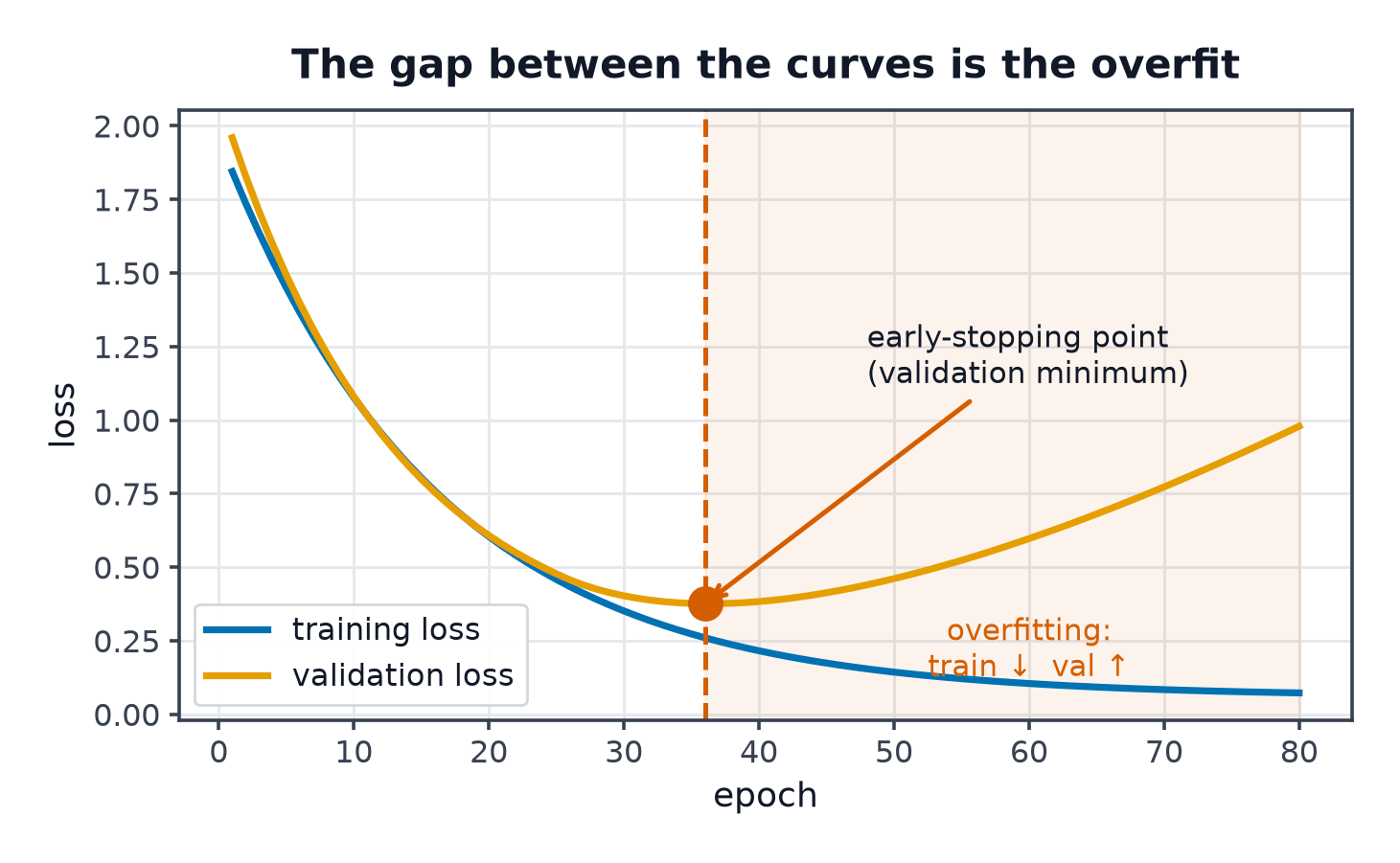
Memorisation vs. generalisation

A model with enough capacity can always achieve zero training error by memorising every training example, including its noise. That is never the goal — the goal is a model that performs well on data it has never seen. The gap between training and validation performance is the direct evidence of how much memorisation is happening (see Bias-Variance Tradeoff).

Detecting overfitting

Track training and validation loss together throughout training. Overfitting shows up as training loss continuing to fall while validation loss flattens or rises — the model is improving its fit to noise it will never see again.

Capacity control

The most direct lever: reduce how expressive the model family is (a shallower tree, fewer parameters, a smaller network). Less capacity means it's physically unable to memorise as much of the training set's idiosyncrasy.

L2 (weight decay)

Add a penalty proportional to squared weight magnitude:

$$L_{\text{total}} = L_{\text{data}} + \lambda \sum_i w_i^2$$

Geometrically, this shrinks all weights toward zero smoothly and proportionally — large weights are pulled down harder than small ones, but nothing is forced to exactly zero.

L1 and sparsity

Why L1 zeroes coefficients and L2 only shrinks them. The solution is where the loss contour first touches the constraint region — the diamond's corners sit on the axes, so contact there sets a coefficient to exactly zero. Both solutions here are solved for, not drawn by eye.

$$L_{\text{total}} = L_{\text{data}} + \lambda \sum_i |w_i|$$

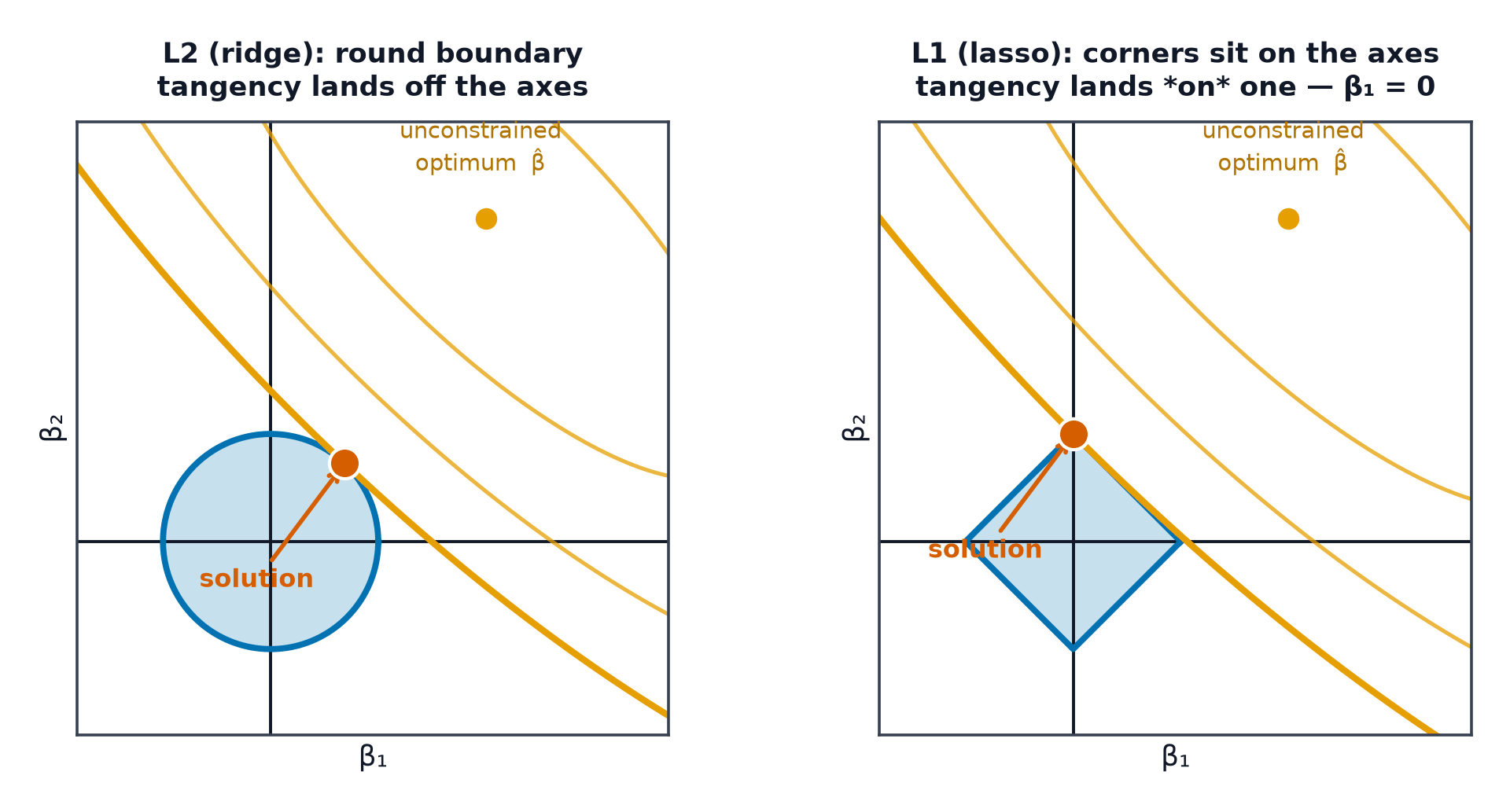
The L1 penalty's constraint region is a diamond (in 2D) rather than L2's circle — the optimum of a smooth loss constrained to a diamond tends to land exactly on a corner, where one or more coordinates are precisely zero. This is why L1 produces sparse solutions (some weights driven to exactly zero, effectively performing feature selection) while L2 only shrinks weights toward — but not to — zero.

Symbol	Meaning
$L_{\text{data}}$	the original task loss (e.g. cross-entropy)
$\lambda$	regularisation strength — how much the penalty matters relative to the data loss
$R(w)$	the penalty term (L1 or L2 norm of the weights)

Elastic net

A weighted combination of both: $R(w) = \alpha \sum_i |w_i| + (1-\alpha) \sum_i w_i^2$ — gets some sparsity from the L1 term and some stability from the L2 term when features are correlated.

Early stopping

Monitor validation loss during training and stop (or restore the best checkpoint) once it stops improving, even if training loss is still falling. This is implicit regularisation: it limits how long the model is allowed to keep memorising.

Data augmentation as regularisation

Synthetically expanding the training set (flips, crops, noise) forces the model to be invariant to those transformations rather than memorising exact pixel values — see Data Augmentation for the full vision-specific treatment.

Dropout, stated

Randomly zero out a fraction of activations during training, forcing the network to not rely on any single unit. Full mechanics and code in Regularization in Deep Nets.

More data as the strongest regulariser

Every technique above is a way of compensating for having too little data relative to model capacity. If you can simply collect more real data, it is usually the single most effective fix — it directly attacks the variance term in the bias-variance decomposition without any of the trade-offs the techniques above introduce.

Selection table

Situation	Reach for
Many correlated features, want stability	L2 / ridge
Want automatic feature selection	L1 / lasso
Both, features correlated and many are irrelevant	elastic net
Training for many epochs, no time to tune capacity	early stopping
Small image/audio/text dataset	data augmentation
Deep network, no other regularisation applied yet	dropout
Any situation, if it's available	more data

Code: ridge and lasso, coefficient paths

regularization_demo.py

import numpy as np
from sklearn.linear_model import Ridge, Lasso
from sklearn.preprocessing import StandardScaler

rng = np.random.default_rng(0)
n, d = 100, 20
X = rng.normal(size=(n, d))
true_w = np.zeros(d)
true_w[:5] = [3, -2, 1.5, 0, 0]  # only first 3 features actually matter
y = X @ true_w + rng.normal(scale=0.5, size=n)

X_scaled = StandardScaler().fit_transform(X)  # mandatory before regularising

lambdas = np.logspace(-2, 2, 10)
print("lambda | ridge nonzero-ish coefs | lasso exact-zero coefs")
for lam in lambdas:
    ridge = Ridge(alpha=lam).fit(X_scaled, y)
    lasso = Lasso(alpha=lam).fit(X_scaled, y)
    ridge_small = np.sum(np.abs(ridge.coef_) < 0.01)
    lasso_zero = np.sum(lasso.coef_ == 0.0)
    print(f"{lam:6.2f} | ridge near-zero: {ridge_small:2d} | lasso exact-zero: {lasso_zero:2d}")

As $\lambda$ grows, lasso's exact-zero count climbs toward $d$ while ridge's coefficients merely shrink — verifying the geometric argument numerically rather than just asserting it.

See also

• Bias-Variance Tradeoff — the theory this page's techniques are fixes for.
• Loss Functions — where the penalty term is added to the objective.