Probability and Distributions

A classifier doesn't output "the answer" — it outputs a belief, expressed as a probability distribution over possible answers. Every loss function in this knowledge base is a statement about how that belief compares to reality. This page is the probability vocabulary everything downstream assumes you already have.

Key idea

A classifier's output is a conditional distribution $p(y \mid x)$, and every loss here is a statement about that distribution.

The distributions that recur throughout ML. The last panel is the central limit theorem in action: averages of uniform samples become normal remarkably quickly, which is why the normal assumption is so often defensible.

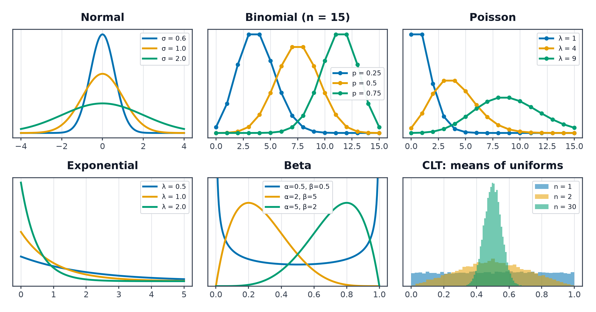
Sample space, events, random variables

The sample space $\Omega$ is the set of all possible outcomes (e.g., all six faces of a die). An event is a subset of $\Omega$ (e.g., "rolled an even number"). A random variable $X$ is a function mapping outcomes to numbers, letting you talk about "the value" rather than "the outcome."

Discrete vs. continuous: PMF, PDF, CDF

• PMF (probability mass function), discrete $X$: $p(x) = P(X = x)$, and $\sum_x p(x) = 1$.
• PDF (probability density function), continuous $X$: $f(x)$ where $P(a \le X \le b) = \int_a^b f(x)\,dx$. Note $f(x)$ is not a probability itself — only the integral over a range is.
• CDF (cumulative distribution function): $F(x) = P(X \le x)$, applies to both.

Expectation and variance

$$\mathbb{E}[X] = \sum_x x \, p(x) \quad \text{(discrete)}, \qquad \mathbb{E}[X] = \int x f(x)\,dx \quad \text{(continuous)}$$ $$\text{Var}(X) = \mathbb{E}\big[(X - \mathbb{E}[X])^2\big]$$

Symbol	Meaning
$\mathbb{E}[X]$	expectation — the long-run average value of $X$
$\text{Var}(X)$	variance — expected squared deviation from the mean

Joint, marginal, conditional

• Joint: $p(x, y)$, the probability of both $X=x$ and $Y=y$.
• Marginal: $p(x) = \sum_y p(x, y)$ — summing out the variable you don't care about.
• Conditional: $p(y \mid x) = \frac{p(x, y)}{p(x)}$ — the distribution of $Y$ once $X$ is known.

Independence

$X$ and $Y$ are independent iff $p(x, y) = p(x)p(y)$ for all $x, y$ — equivalently, knowing $X$ tells you nothing about $Y$. This assumption is the backbone of Naive Bayes, and it's usually false — which is exactly why that page is interesting.

Bayes' rule

$$p(y \mid x) = \frac{p(x \mid y)\, p(y)}{p(x)}$$

Worked example (the base-rate trap): a disease affects 1% of the population; a test is 99% accurate (both sensitivity and specificity). Given a positive test, what's the probability of actually having the disease?

$$p(\text{disease} \mid \text{positive}) = \frac{0.99 \times 0.01}{0.99 \times 0.01 + 0.01 \times 0.99} = 0.5$$

Only 50%, not 99% — because the disease is rare, false positives from the healthy 99% of the population outnumber true positives from the sick 1%. Ignoring the base rate $p(y)$ is the single most common probability mistake in applied ML.

The distributions that matter

Distribution	Support	Use
Bernoulli	$\{0, 1\}$	a single binary outcome (coin flip, binary label)
Categorical	$\{1, \ldots, K\}$	a single outcome among $K$ classes
Gaussian (Normal)	$\mathbb{R}$	continuous data, noise, weight initialisation
Uniform	$[a, b]$	"no prior preference" over a range
Exponential	$[0, \infty)$	waiting times, time-to-event

The Gaussian's special status

The Gaussian $\mathcal{N}(\mu, \sigma^2)$ has PDF $f(x) = \frac{1}{\sigma\sqrt{2\pi}} e^{-\frac{(x-\mu)^2}{2\sigma^2}}$. It arises constantly because of the central limit theorem: the sum (or mean) of many independent random variables tends toward a Gaussian, regardless of their original distribution — which is why noise, measurement error, and aggregated effects are so often modelled as Gaussian.

Code: sampling, plotting, and an empirical CLT demo

distributions_demo.py

import numpy as np
import matplotlib.pyplot as plt

rng = np.random.default_rng(0)

# --- Sample from each named distribution ---
bernoulli = rng.binomial(1, p=0.3, size=1000)
categorical = rng.choice([0, 1, 2], p=[0.5, 0.3, 0.2], size=1000)
gaussian = rng.normal(loc=0, scale=1, size=1000)
uniform = rng.uniform(low=-1, high=1, size=1000)
exponential = rng.exponential(scale=1.0, size=1000)

print("bernoulli mean:", bernoulli.mean())
print("gaussian mean/std:", gaussian.mean(), gaussian.std())

# --- Empirical central limit theorem ---
n_samples, n_sums = 10000, 30
uniform_sums = rng.uniform(0, 1, size=(n_samples, n_sums)).sum(axis=1)

fig, axes = plt.subplots(1, 2, figsize=(10, 4))
axes[0].hist(rng.uniform(0, 1, n_samples), bins=50)
axes[0].set_title("single uniform draw")
axes[1].hist(uniform_sums, bins=50)
axes[1].set_title(f"sum of {n_sums} uniform draws (bell-shaped)")
plt.savefig("clt_demo.png")

Summing 30 uniform draws already looks visibly bell-shaped despite the uniform distribution having no bell shape at all — the CLT in action.

See also

• Statistics and Estimation — using these distributions to estimate parameters from data.
• Information Theory — measuring surprise and divergence between distributions.