Statistics and Estimation

Fitting a model is estimating parameters from a finite sample — and every estimate comes with uncertainty about how wrong it might be. This page derives maximum likelihood estimation, the principle underlying nearly every loss function used in this knowledge base, and shows the bridge from "most likely parameters" to "squared error" and "cross-entropy."

Key idea

Nearly every loss function in ML is a negative log-likelihood in disguise.

Standard error shrinks as 1/√n, so quartering your error costs sixteen times the data. On the right, '95 % confident' describes the procedure: run it many times and about 95 % of the intervals it produces will contain the truth.

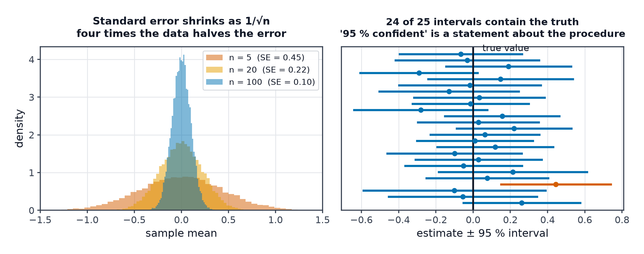
Population vs. sample

The population is the entire (often infinite, unobservable) set of things you care about; the sample is the finite subset you actually observed. Every statistic computed from a sample is an estimate of some population quantity, not the quantity itself.

Estimators: bias, variance, consistency

An estimator $\hat\theta$ is a function of the sample used to guess a population parameter $\theta$.

• Bias: $\text{Bias}(\hat\theta) = \mathbb{E}[\hat\theta] - \theta$ — systematic error, present even with infinite data of the same sample size.
• Variance: how much $\hat\theta$ fluctuates across different samples.
• Consistency: $\hat\theta \to \theta$ as sample size $\to \infty$.

Maximum likelihood estimation

Given a model family $p(x \mid \theta)$ and observed data $x_1, \ldots, x_n$ (assumed i.i.d.), the likelihood is how probable the data is under a given $\theta$:

$$L(\theta) = \prod_{i=1}^n p(x_i \mid \theta)$$

MLE picks the $\theta$ that makes the observed data most probable: $\hat\theta_{\text{MLE}} = \arg\max_\theta L(\theta)$. In practice you maximise the log-likelihood instead (same maximiser, numerically stable, turns a product into a sum):

$$\ell(\theta) = \log L(\theta) = \sum_{i=1}^n \log p(x_i \mid \theta)$$

MLE for a Gaussian, derived

Assume $x_i \sim \mathcal{N}(\mu, \sigma^2)$. The log-likelihood is:

$$\ell(\mu, \sigma^2) = -\frac{n}{2}\log(2\pi\sigma^2) - \frac{1}{2\sigma^2}\sum_i (x_i - \mu)^2$$

Setting $\frac{\partial \ell}{\partial \mu} = 0$ gives $\hat\mu_{\text{MLE}} = \frac{1}{n}\sum_i x_i$ — the sample mean. Setting $\frac{\partial \ell}{\partial \sigma^2} = 0$ gives $\hat\sigma^2_{\text{MLE}} = \frac{1}{n}\sum_i (x_i - \hat\mu)^2$ — the (biased) sample variance.

MLE for Bernoulli

For $x_i \in \{0, 1\}$ with $p(x_i = 1) = \theta$: $\ell(\theta) = \sum_i \big[x_i \log\theta + (1-x_i)\log(1-\theta)\big]$, maximised at $\hat\theta = \frac{1}{n}\sum_i x_i$ — the observed fraction of ones.

From MLE to squared error and cross-entropy

This is the key bridge. If you assume regression targets have Gaussian noise, $y_i \sim \mathcal{N}(f(x_i), \sigma^2)$, maximising the log-likelihood over $f$'s parameters is exactly minimising $\sum_i (y_i - f(x_i))^2$ — squared error. If you assume a Bernoulli output for classification, maximising the log-likelihood over the model's parameters is exactly minimising binary cross-entropy. The loss functions in Loss Functions are not arbitrary choices — they are MLE under specific noise assumptions.

Symbol	Meaning
$L(\theta)$	likelihood of the data given parameters $\theta$
$\ell(\theta)$	log-likelihood
$\hat\theta_{\text{MLE}}$	the maximum likelihood estimate

MAP and priors

Maximum a posteriori adds a prior belief $p(\theta)$ over parameters before seeing data: $\hat\theta_{\text{MAP}} = \arg\max_\theta \big[\log p(x \mid \theta) + \log p(\theta)\big]$. A Gaussian prior on weights, worked through, produces exactly the L2 regularisation term in Overfitting and Regularization — regularisation is MAP estimation with a specific prior.

Confidence intervals and bootstrap

A confidence interval expresses the estimate's uncertainty: "the true value is in this range, with this confidence, under repeated sampling." The bootstrap estimates this without any distributional assumption: resample the data (with replacement) many times, recompute the statistic each time, and use the spread of results as the uncertainty estimate.

Hypothesis testing, honestly

A p-value is the probability of seeing data this extreme if the null hypothesis were true — it is not the probability the null hypothesis is true, and repeated testing without correction inflates false positives. In ML practice, hypothesis tests appear most often in A/B testing (see Online Evaluation and A/B Testing); treat p-value thresholds as one input to a decision, not a verdict.

Code: MLE by hand, and a bootstrap confidence interval

mle_and_bootstrap.py

import numpy as np

rng = np.random.default_rng(0)
data = rng.normal(loc=5.0, scale=2.0, size=200)

# --- MLE for a Gaussian, by hand vs. NumPy ---
mu_hat = data.sum() / len(data)
sigma2_hat = ((data - mu_hat) ** 2).sum() / len(data)
print(f"hand-derived MLE: mu={mu_hat:.3f}, sigma^2={sigma2_hat:.3f}")
print(f"numpy:            mu={data.mean():.3f}, sigma^2={data.var():.3f}")

# --- Bootstrap confidence interval for a model's accuracy ---
def fake_model_accuracy(sample):
    """Stand-in for a real evaluation metric computed on a resampled test set."""
    return (sample > 4.5).mean()

n_boot = 2000
boot_scores = np.array([
    fake_model_accuracy(rng.choice(data, size=len(data), replace=True))
    for _ in range(n_boot)
])
lo, hi = np.percentile(boot_scores, [2.5, 97.5])
print(f"bootstrap 95% CI for the metric: [{lo:.3f}, {hi:.3f}]")

See also

• Loss Functions — where MLE cashes out into the losses actually trained against.
• Probability and Distributions — the distributions MLE is estimating parameters for.