Autoencoders

Train a network to copy its input to its output, and the task sounds trivially easy — the identity function does it perfectly. Force that copying to pass through a narrow bottleneck first, and suddenly the network has to decide what matters enough to keep. That forced compression is the entire idea behind autoencoders.

Key idea

Forcing reconstruction through a narrow layer makes the network learn what matters and discard what does not - it is non-linear compression.

An autoencoder is trained only to reproduce its input. The bottleneck is what forces it to learn a compressed representation rather than the identity function — and a plain autoencoder's latent space has no structure that makes sampling meaningful.

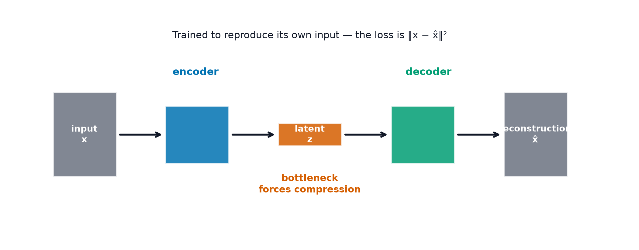
The encoder-bottleneck-decoder shape

An encoder compresses the input $x$ into a lower-dimensional latent representation $z$; a decoder reconstructs an approximation $\hat x$ from $z$ alone. The bottleneck's width (the dimensionality of $z$) is the key architectural choice — narrower forces more aggressive compression.

Reconstruction loss

$$L = \|x - \hat x\|^2$$

Simple squared error between input and reconstruction, exactly Loss Functions's MSE — the training objective is purely "reconstruct well," with nothing explicitly telling the network what to keep, only implicitly forcing a choice via the bottleneck's limited capacity.

The relationship to PCA

A linear autoencoder (no non-linear activations, squared-error loss) provably learns to span the same subspace as PCA and SVD's top principal components — a striking connection showing PCA is, in this specific sense, a special case of autoencoding. A non-linear autoencoder generalises this to non-linear manifolds that PCA's linear projection cannot capture.

Symbol	Meaning
$x$	the input
$z$	the latent (bottleneck) representation
$\hat x$	the reconstruction

Undercomplete vs. overcomplete

Undercomplete: bottleneck dimension smaller than the input — forces genuine compression, the standard setting. Overcomplete: bottleneck dimension equal to or larger than the input — without another constraint, an overcomplete autoencoder can trivially learn the identity function and copy every value through unchanged, learning nothing useful; some additional regularisation (sparsity, noise) is required to make an overcomplete autoencoder do anything meaningful.

Denoising autoencoders

Corrupt the input (add noise, randomly zero out some values) before feeding it to the encoder, but require the decoder to reconstruct the original, uncorrupted input — forces the network to learn robust, general features rather than merely memorising exact pixel values, since the exact corrupted input is never actually the reconstruction target.

Sparse autoencoders

Add a penalty encouraging most latent units to be near-zero for any given input, even in an overcomplete setting — rather than forcing compression via bottleneck width, forces it via bottleneck sparsity (few active units per example), a different mechanism achieving a related effect.

Contractive autoencoders, briefly

Penalise the sensitivity of the latent representation to small input perturbations directly (the norm of the encoder's Jacobian) — encourages the encoder to be locally flat/robust around real data points, a more direct mathematical statement of "learn robust features" than denoising's noise-injection approach.

What the latent space looks like, and why it's not smooth

Nothing in a plain autoencoder's training objective constrains the latent space's overall structure — only that specific training points, once encoded, decode back correctly. This means the latent space can have gaps, discontinuities, and regions with no correspondence to any real data at all, between the specific points the network happened to see during training.

Why you cannot sample from a plain autoencoder

To generate a new sample, you'd need to pick some $z$ and decode it — but since the latent space has no known, well-behaved overall structure, there's no principled way to choose a "good" $z$ that will decode to something realistic. Decoding a random point is likely to land in one of the latent space's unstructured gaps, producing garbage. This exact gap is what Variational Autoencoders fixes directly, by forcing the latent space into a known, well-behaved distribution.

Real uses

Anomaly detection: train on normal data only; a point that reconstructs poorly (high reconstruction error) is, by that measure, anomalous — connecting to Anomaly Detection's reconstruction-error method. Compression: the encoder's output is a compressed representation. Pretraining: use the trained encoder as a feature extractor for a downstream task. Dimensionality reduction: the non-linear generalisation of PCA and SVD.

Code: autoencoder on MNIST-scale data, latent space gaps, decoding noise

autoencoders_demo.py

import torch
import torch.nn as nn
from torchvision import datasets, transforms
import matplotlib.pyplot as plt

class Autoencoder(nn.Module):
    def __init__(self, bottleneck_dim):
        super().__init__()
        self.encoder = nn.Sequential(nn.Flatten(), nn.Linear(784, 128), nn.ReLU(), nn.Linear(128, bottleneck_dim))
        self.decoder = nn.Sequential(nn.Linear(bottleneck_dim, 128), nn.ReLU(), nn.Linear(128, 784), nn.Sigmoid())
    def forward(self, x):
        z = self.encoder(x)
        return self.decoder(z).view(-1, 1, 28, 28), z

transform = transforms.ToTensor()
train_data = datasets.MNIST(root="./data", train=True, download=True, transform=transform)
loader = torch.utils.data.DataLoader(train_data, batch_size=128, shuffle=True)

fig, axes = plt.subplots(2, 3, figsize=(9, 6))
for row, bottleneck_dim in enumerate([2, 32]):
    model = Autoencoder(bottleneck_dim)
    optimizer = torch.optim.Adam(model.parameters(), lr=0.001)
    for epoch in range(3):
        for x, _ in loader:
            optimizer.zero_grad()
            recon, z = model(x)
            loss = nn.functional.mse_loss(recon, x)
            loss.backward(); optimizer.step()

    x_sample, _ = next(iter(loader))
    recon, z = model(x_sample[:1])
    axes[row, 0].imshow(x_sample[0, 0], cmap="gray"); axes[row, 0].set_title(f"original (dim={bottleneck_dim})")
    axes[row, 1].imshow(recon[0, 0].detach(), cmap="gray"); axes[row, 1].set_title("reconstruction")

    if bottleneck_dim == 2:
        random_z = torch.randn(1, 2)  # decode a random point in the 2-D latent space
        random_decode = model.decoder(random_z).view(28, 28)
        axes[row, 2].imshow(random_decode.detach(), cmap="gray")
        axes[row, 2].set_title("decoding a RANDOM latent point\n(often not a recognisable digit)")
plt.savefig("autoencoder_reconstructions.png")

See also

• PCA and SVD — the linear special case autoencoders provably generalise.
• Variational Autoencoders — the probabilistic fix that makes sampling from the latent space actually work.