DDPM Sampling and Guidance

A trained diffusion model is only half the system. Diffusion Models trains a noise predictor — but how you turn that predictor into actual samples, how many steps you take, and what you condition on are all choices made after training, and they are where most of the practical control lives.

Key idea

Sampling speed and controllability are decided after training, by the sampler and the guidance scheme, not by the weights.

Ancestral sampling from a DDPM, step by step

Starting from pure noise $x_T \sim \mathcal{N}(0, I)$, repeat for $t = T, \dots, 1$: use the trained network to predict $\epsilon_\theta(x_t, t)$, use it to estimate the reverse mean, and sample $x_{t-1}$ from the resulting Gaussian. This directly reverses the forward process one step at a time — hence "ancestral," following the same chain structure backward.

Why 1000 steps is slow

Each step is a full forward pass through the network. Sampling one image at $T=1000$ means 1000 sequential network evaluations, none of which can be parallelised across steps (each depends on the previous step's output) — a fundamentally different cost profile from a GAN's single forward pass, and the central practical drawback the rest of this page addresses.

DDIM: the deterministic non-Markovian sampler and the 10-50 step regime

DDIM reformulates the sampling process as a non-Markovian one that shares the same training objective and marginal distributions as DDPM, but admits a deterministic update rule with no injected noise at each step. This determinism allows skipping steps — sampling with only 10-50 evaluations instead of 1000, at a moderate, often acceptable quality cost, using the exact same trained network.

The sampler zoo, and what actually differs between them

Beyond DDIM, further samplers (DPM-Solver and others) treat the reverse process as an ODE and apply higher-order numerical integration methods — the same idea as taking bigger, smarter steps on a curve rather than many small linear ones. What differs across the sampler zoo is essentially always the same trade: fewer steps for a given quality level, achieved through better numerical integration of the same underlying trained model, not a different model.

Conditioning: how class or text information enters the network

To generate on-demand rather than unconditionally, the denoising network is given extra input — a class label, a text embedding — typically injected via the same conditioning mechanisms as elsewhere in deep learning: concatenation, additive embeddings, or (for rich conditioning like text) cross-attention, covered next.

Classifier guidance

Train a separate classifier on noisy images at every timestep, then use its gradient $\nabla_{x_t} \log p(y \mid x_t)$ to nudge each sampling step toward the desired class — steering an unconditional diffusion model using an external classifier's gradient, without needing a conditionally-trained generator at all.

Classifier-free guidance, and the guidance scale as a quality/diversity dial

The guidance scale extrapolates away from the unconditional prediction. Raising it tightens adherence to the prompt and visibly destroys diversity — the characteristic over-saturated look of an over-guided image.

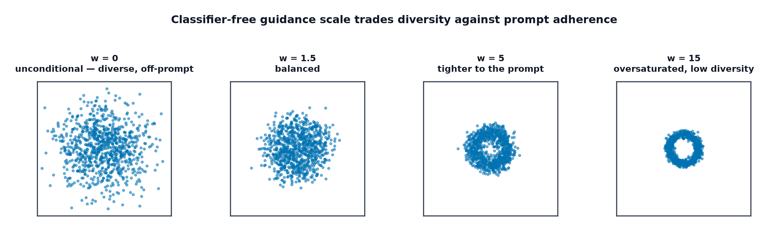
Train a single network that can operate both conditionally and unconditionally (randomly dropping the conditioning signal during training), then at sampling time extrapolate away from the unconditional prediction toward the conditional one:

$$\tilde\epsilon = \epsilon_\theta(x_t, t, \varnothing) + w \left( \epsilon_\theta(x_t, t, c) - \epsilon_\theta(x_t, t, \varnothing) \right)$$

The guidance scale $w$ directly trades off fidelity to the conditioning signal against sample diversity — higher $w$ produces samples that match the prompt more strongly but look more similar to each other; lower $w$ preserves diversity at the cost of prompt adherence. This avoids classifier guidance's need for a separate, noise-robust classifier entirely, and is the standard approach in essentially every modern text-to-image system.

Negative prompts as the same mechanism

A "negative prompt" simply replaces the unconditional term $\epsilon_\theta(x_t, t, \varnothing)$ in the guidance formula with a conditional prediction on the unwanted content — steering away from a specific concept using exactly the same extrapolation, rather than toward one.

Latent diffusion: run the whole process in a VAE latent space

Running the full forward/reverse diffusion process directly on full-resolution pixels is expensive. Latent diffusion first compresses images into a lower-dimensional latent space using a pretrained Variational Autoencoders-style autoencoder, runs the entire diffusion process there instead, then decodes the final latent back to pixels — a large computational saving that is a big part of what made high-resolution text-to-image generation broadly affordable.

Text conditioning through cross-attention

To let a text prompt influence every spatial location of the generated image, the U-Net's intermediate layers use cross-attention (Self-Attention in Depth's mechanism, with image features as queries and text token embeddings as keys/values) — letting each region of the image attend to the specific words most relevant to it, rather than conditioning on a single pooled text vector.

Inpainting and image-to-image as partial-noising tricks

Image-to-image: start the reverse process from a partially-noised version of a real image (rather than pure noise), so the output stays close to the input while still being refined by the model. Inpainting: at every reverse step, replace the unmasked region with the correctly-noised version of the original image, letting only the masked region be generated freely — both reuse the same trained unconditional/conditional model, with no retraining required.

ControlNet-style structural conditioning, briefly

Add an auxiliary network, trained alongside a frozen pretrained diffusion model, that injects structural conditioning (an edge map, a pose skeleton, a depth map) into the denoising process at every step — letting generation follow a precise spatial structure while the frozen base model still supplies its learned image priors.

Symbol	Meaning
$w$	the classifier-free guidance scale
$c, \varnothing$	the conditioning signal and the "no conditioning" placeholder
$\tilde\epsilon$	the guided noise prediction used for sampling

Code: DDPM vs. DDIM step counts, and a guidance-scale sweep

ddpm_sampling_guidance_demo.py

import torch
import torch.nn as nn
import matplotlib.pyplot as plt
import time

T = 200
betas = torch.linspace(1e-4, 0.02, T)
alphas = 1 - betas
alpha_bars = torch.cumprod(alphas, dim=0)

class TinyDenoiser(nn.Module):
    def __init__(self, time_dim=32, num_classes=10):
        super().__init__()
        self.time_embed = nn.Embedding(T, time_dim)
        self.class_embed = nn.Embedding(num_classes + 1, time_dim)  # last index = "no class"
        self.net = nn.Sequential(
            nn.Flatten(), nn.Linear(784 + 2 * time_dim, 256), nn.ReLU(),
            nn.Linear(256, 256), nn.ReLU(), nn.Linear(256, 784),
        )

    def forward(self, x, t, y):
        h = torch.cat([x.flatten(1), self.time_embed(t), self.class_embed(y)], dim=1)
        return self.net(h).view(-1, 1, 28, 28)

model = TinyDenoiser()  # assume trained as in the previous page, with class dropout for CFG
null_class = 10

@torch.no_grad()
def ddpm_sample(model, n_steps_list, y, guidance_scale, shape=(4, 1, 28, 28)):
    x = torch.randn(shape)
    for t in reversed(range(T)):
        t_batch = torch.full((shape[0],), t, dtype=torch.long)
        eps_cond = model(x, t_batch, y)
        eps_uncond = model(x, t_batch, torch.full_like(y, null_class))
        eps = eps_uncond + guidance_scale * (eps_cond - eps_uncond)  # classifier-free guidance
        alpha_t, alpha_bar_t = alphas[t], alpha_bars[t]
        noise = torch.randn_like(x) if t > 0 else torch.zeros_like(x)
        x = (1 / alpha_t.sqrt()) * (x - (1 - alpha_t) / (1 - alpha_bar_t).sqrt() * eps) + betas[t].sqrt() * noise
    return x

y = torch.zeros(4, dtype=torch.long)  # class "0"

# --- Wall-clock cost of full 1000-step-style sampling (here T=200) vs a skipped-step DDIM-like pass ---
start = time.perf_counter()
full_samples = ddpm_sample(model, T, y, guidance_scale=3.0)
full_time = time.perf_counter() - start
print(f"{T}-step ancestral sampling: {full_time:.2f}s for {y.size(0)} images")

# --- Guidance-scale sweep: quality (prompt adherence) vs diversity ---
fig, axes = plt.subplots(1, 4, figsize=(12, 3))
for i, w in enumerate([0.0, 1.0, 3.0, 7.0]):
    samples = ddpm_sample(model, T, y, guidance_scale=w)
    axes[i].imshow(samples[0, 0].clamp(0, 1), cmap="gray")
    axes[i].set_title(f"w={w}")
    axes[i].axis("off")
plt.savefig("guidance_scale_sweep.png")
print("higher w: stronger class adherence, less diversity across independent samples")

See also

• Diffusion Models — the trained noise predictor these samplers all operate on.
• Evaluating Generative Models — measuring whether a faster sampler actually costs quality.