Diffusion Models

Generating an image from nothing in one shot is hard. Diffusion sidesteps the difficulty entirely: destroy an image with noise across many small steps, then train a network to undo just one of those small steps at a time — a thousand easy problems standing in for one hard one.

Key idea

Learning to remove a little noise is easy; iterating that easy problem a thousand times solves the hard problem of generating from nothing.

The forward process destroys structure with noise on a fixed schedule and requires no learning at all. The model learns only to undo one step — and chaining those small reversals from pure noise is what generates a sample.

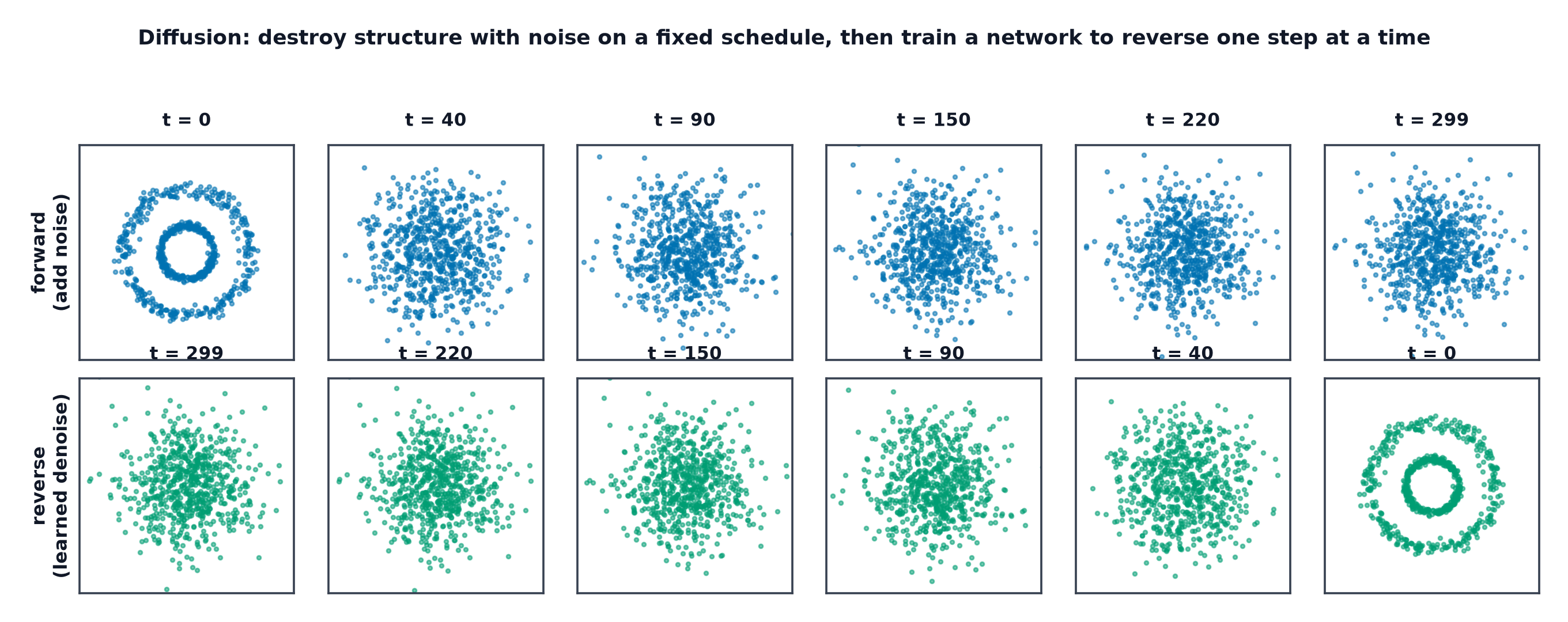
The intuition: a hard problem decomposed into many easy ones

Predicting a clean image directly from pure noise requires the network to somehow invent all of an image's structure in one step. Predicting slightly less noisy from slightly more noisy, repeated a thousand times, only ever asks the network to do a small, local correction — a far easier learning problem, and the entire reason diffusion works at all.

The forward process: fixed, no learning, Gaussian noise on a schedule

The forward process $q(x_t \mid x_{t-1})$ adds a small, fixed amount of Gaussian noise at every step $t = 1, \dots, T$:

$$q(x_t \mid x_{t-1}) = \mathcal{N}(x_t;\ \sqrt{1 - \beta_t}\, x_{t-1},\ \beta_t I)$$

Nothing here is learned — $\beta_t$ is a fixed schedule chosen in advance, and by $t = T$, $x_T$ is (by construction) indistinguishable from pure noise $\mathcal{N}(0, I)$.

The closed form that jumps to any timestep t in one step

Because each forward step is Gaussian, the composition of all steps up to $t$ is also Gaussian, with a closed form that requires no iteration:

$$q(x_t \mid x_0) = \mathcal{N}(x_t;\ \sqrt{\bar\alpha_t}\, x_0,\ (1 - \bar\alpha_t) I), \qquad \bar\alpha_t = \prod_{i=1}^t (1 - \beta_i)$$

This closed form is what makes training practical: given a clean image $x_0$ and any timestep $t$, you can sample a noised $x_t$ directly, without simulating all $t$ forward steps.

Noise schedules and what they change

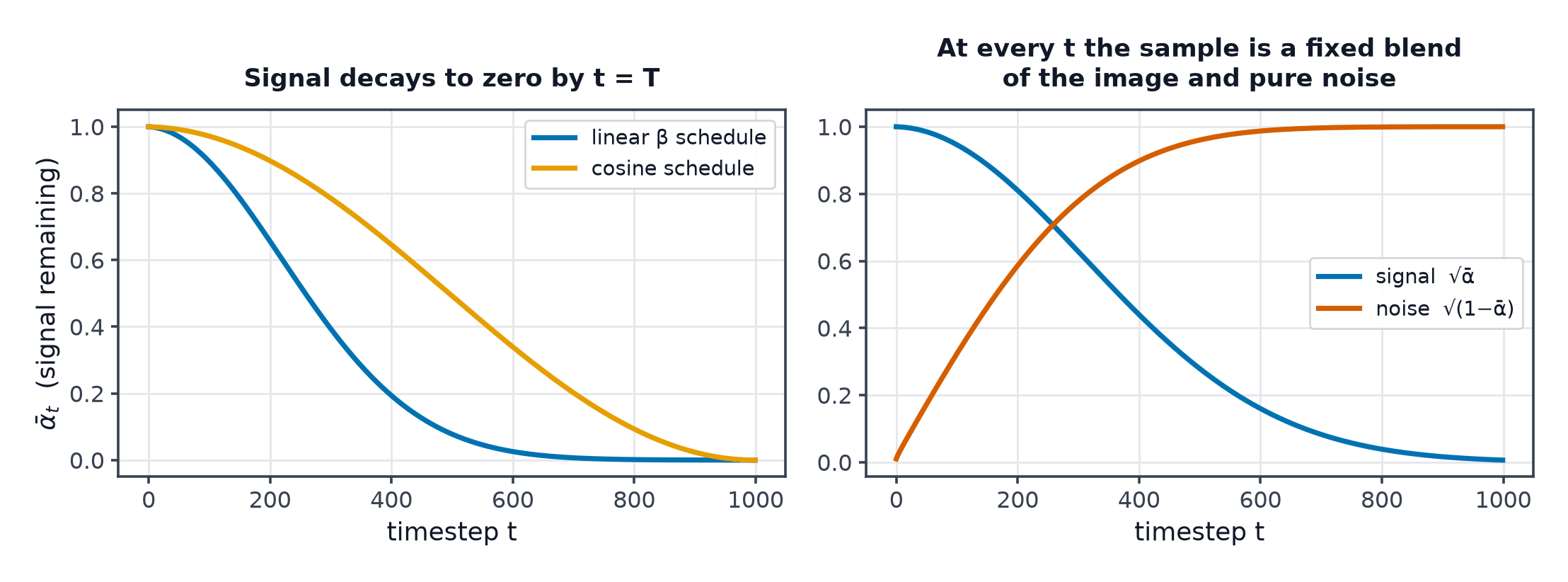
The schedule fixes how much signal survives at each timestep. The linear schedule destroys information too early in the trajectory, which is why the cosine schedule replaced it for image models.

Linear schedule: $\beta_t$ increases linearly from a small value to a larger one across the $T$ steps — the original DDPM choice. Cosine schedule: shaped to add noise more gradually near $t=0$ and $t=T$, which empirically improves sample quality, particularly at lower step counts — the schedule directly controls how much "signal" remains at each intermediate timestep, and a badly-chosen schedule can waste steps where noise is added too fast to be useful for learning.

The reverse process: the learned part

The reverse process $p_\theta(x_{t-1} \mid x_t)$ is a neural network's approximation of "undo one forward step" — this is the only part of the whole system with trainable parameters. Since the forward process is fixed and known, the reverse process's target is entirely determined by that forward process's mathematics, not by anything hand-designed.

What the network actually predicts, and why that parameterisation won

In principle the network could predict the clean image $x_0$ directly, or the mean of the reverse distribution — but the DDPM paper found that reparameterising the network to predict the noise $\epsilon$ that was added (rather than the denoised image itself) produces a simpler, better-behaved training signal empirically, and this $\epsilon$-prediction parameterisation is what nearly all subsequent diffusion work has kept.

The simplified training objective

$$L_{\text{simple}} = \mathbb{E}_{t, x_0, \epsilon} \left[ \|\epsilon - \epsilon_\theta(x_t, t)\|^2 \right]$$

A plain mean-squared error between the true noise $\epsilon$ that was added and the network's prediction $\epsilon_\theta$ — exactly Loss Functions's MSE, applied to a noise-prediction target rather than a label.

The training loop: sample an image, sample a timestep, add noise, predict it

1. Sample a real image $x_0$ from the training set.
2. Sample a random timestep $t \sim \text{Uniform}(1, T)$.
3. Sample noise $\epsilon \sim \mathcal{N}(0, I)$ and form $x_t$ using the closed-form formula above.
4. Have the network predict $\epsilon$ from $(x_t, t)$; take a gradient step on the MSE.

Notice this never requires simulating the reverse process during training at all — every training step is a single, independent forward computation.

The U-Net backbone with timestep conditioning

The network $\epsilon_\theta(x_t, t)$ is almost universally a U-Net (Semantic and Instance Segmentation's architecture) — image-in, image-out, with the timestep $t$ injected into every block (typically via a sinusoidal embedding added to the feature maps, the same positional-encoding idea from Positional Encodings), so a single network can denoise at every noise level rather than needing $T$ separate networks.

Why diffusion beat GANs on quality and coverage

Diffusion training is a straightforward supervised regression problem (predict the noise), with none of GAN Training Challenges's two-network instability — no mode collapse mechanism, no discriminator/generator balance to tune. Empirically this stability, combined with the iterative refinement process, has produced both higher sample quality and better mode coverage than GANs on large-scale image generation, at the cost described next.

The cost: many forward passes per sample

Generating one sample requires running the reverse process for (up to) $T$ steps sequentially — often hundreds to a thousand network evaluations for a single image, dramatically slower than a GAN's single forward pass. This sampling-speed cost is the direct motivation for DDPM Sampling and Guidance's faster samplers and Flow Matching and Consistency Models's few-step alternatives.

Symbol	Meaning
$x_0, x_t, x_T$	the clean image, image at timestep $t$, and pure noise
$\beta_t, \bar\alpha_t$	the noise schedule and its cumulative product
$\epsilon, \epsilon_\theta$	the true added noise and the network's noise prediction

Code: the forward process visualised, and a small DDPM trained on MNIST-scale data

diffusion_models_demo.py

import torch
import torch.nn as nn
from torchvision import datasets, transforms
import matplotlib.pyplot as plt

T = 200
betas = torch.linspace(1e-4, 0.02, T)
alphas = 1 - betas
alpha_bars = torch.cumprod(alphas, dim=0)

def forward_diffusion(x0, t, noise):
    ab = alpha_bars[t].view(-1, 1, 1, 1)
    return ab.sqrt() * x0 + (1 - ab).sqrt() * noise

transform = transforms.ToTensor()
train_data = datasets.MNIST(root="./data", train=True, download=True, transform=transform)
loader = torch.utils.data.DataLoader(train_data, batch_size=128, shuffle=True)

# --- Visualise the forward process on one image at ten timesteps ---
x0, _ = train_data[0]
x0 = x0.unsqueeze(0)
fig, axes = plt.subplots(1, 10, figsize=(20, 2))
for i, t in enumerate(torch.linspace(0, T - 1, 10).long()):
    noise = torch.randn_like(x0)
    xt = forward_diffusion(x0, t, noise)
    axes[i].imshow(xt[0, 0].clamp(0, 1), cmap="gray"); axes[i].axis("off")
    axes[i].set_title(f"t={t.item()}")
plt.savefig("diffusion_forward_process.png")

# --- A small noise-prediction network, timestep conditioning via embedding ---
class TinyDenoiser(nn.Module):
    def __init__(self, time_dim=32):
        super().__init__()
        self.time_embed = nn.Embedding(T, time_dim)
        self.net = nn.Sequential(
            nn.Flatten(),
            nn.Linear(784 + time_dim, 256), nn.ReLU(),
            nn.Linear(256, 256), nn.ReLU(),
            nn.Linear(256, 784),
        )

    def forward(self, x, t):
        t_emb = self.time_embed(t)
        h = torch.cat([x.flatten(1), t_emb], dim=1)
        return self.net(h).view(-1, 1, 28, 28)

model = TinyDenoiser()
optimizer = torch.optim.Adam(model.parameters(), lr=0.001)
for epoch in range(3):
    total_loss = 0.0
    for x0_batch, _ in loader:
        t = torch.randint(0, T, (x0_batch.size(0),))
        noise = torch.randn_like(x0_batch)
        xt = forward_diffusion(x0_batch, t, noise)
        pred_noise = model(xt, t)
        loss = nn.functional.mse_loss(pred_noise, noise)  # the simplified DDPM objective
        optimizer.zero_grad(); loss.backward(); optimizer.step()
        total_loss += loss.item()
    print(f"epoch {epoch}: mean noise-prediction MSE = {total_loss / len(loader):.4f}")

See also

• DDPM Sampling and Guidance — turning this trained noise predictor into fast, controllable samples.
• Semantic and Instance Segmentation — the U-Net architecture diffusion models build on.