GAN Training Challenges

GANs are famously hard to train, and the failure modes are specific and recognisable. Worse: the standard debugging instinct — watch the loss curve — actively misleads here.

Key idea

Adversarial training has no single loss to monitor - the losses can look fine while the model produces one image forever.

Mode collapse: the generator finds a small set of outputs the discriminator cannot reject and stops exploring. The loss curves can look entirely healthy while this happens, which is why GAN evaluation needs coverage metrics rather than loss.

Why the loss curves tell you almost nothing

In supervised learning, a falling loss means the model is improving. In Generative Adversarial Networks, $D$'s and $G$'s losses are each defined relative to the other, currently-changing network — a generator loss can fall simply because the discriminator got weaker, not because sample quality improved. Two networks chasing a moving target produces loss curves that oscillate, plateau, or look deceptively stable while the actual samples are garbage.

Mode collapse: symptom, cause, diagnostics

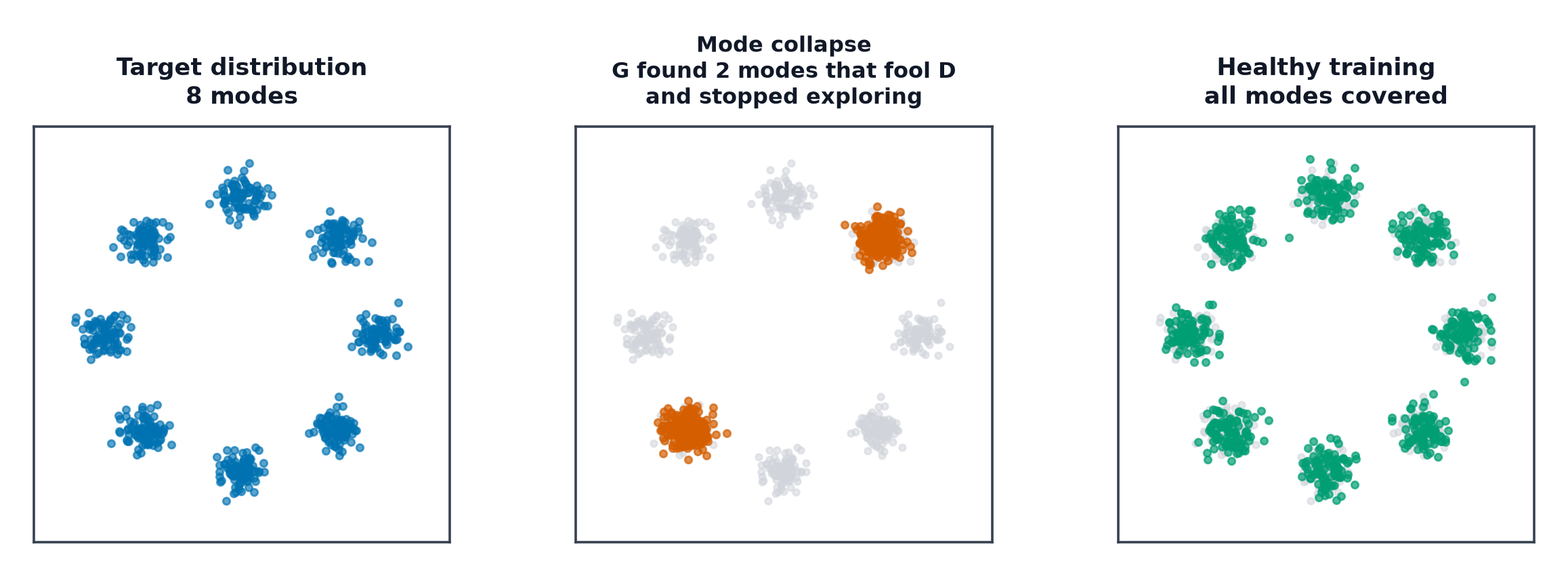
Symptom: the generator produces only a small subset of the true data's diversity — sometimes literally one output, regardless of the input noise $z$. Cause: if $G$ finds a single output that reliably fools the current $D$, gradient descent has no built-in pressure to keep exploring — collapsing to that one mode can be a stable equilibrium of the minimax game as actually optimised (as opposed to the idealised simultaneous optimum). Diagnostics: plot generated samples across training steps side by side (not just the final result); a healthy run's samples keep varying, a collapsed run's samples visually converge to near-duplicates.

Vanishing discriminator gradients when the discriminator wins

If $D$ becomes too good too early, $D(G(z)) \approx 0$ for essentially all generated samples — and the original (saturating) generator loss $\log(1 - D(G(z)))$ has near-zero gradient in exactly that regime, exactly when $G$ most needs a signal. This is precisely why Generative Adversarial Networks's non-saturating loss ($-\log D(G(z))$) is used instead of the literal minimax formulation in practice.

Oscillation and non-convergence

Because both networks update in response to a target that keeps moving, standard gradient descent has no guarantee of converging to the minimax equilibrium at all — the pair can cycle indefinitely (generator produces mode A, discriminator learns to reject A, generator switches to mode B, discriminator learns to reject B, generator switches back to A) instead of settling.

The balance problem between the two networks

If $D$ is much stronger than $G$: vanishing gradients, as above. If $G$ is much stronger than $D$: $D$ never learns a meaningful decision boundary, and its feedback to $G$ becomes uninformative noise. Neither imbalance is fixed simply by "training the weaker one more" — the interaction is what needs tuning, not either network in isolation.

Wasserstein GAN: the earth-mover motivation and the critic reformulation

WGAN replaces the original $D$'s real/fake probability output with a critic that outputs an unbounded real-valued score, trained to approximate the Wasserstein (earth-mover) distance between the real and generated distributions — a distance metric that, unlike the original GAN's Jensen-Shannon-based objective, stays meaningful (non-zero, with useful gradients) even when the two distributions have little or no overlap, which is exactly the regime early GAN training operates in.

$$W(p_{\text{data}}, p_g) = \sup_{\|f\|_L \leq 1} \; \mathbb{E}_{x \sim p_{\text{data}}}[f(x)] - \mathbb{E}_{x \sim p_g}[f(x)]$$

Weight clipping and its problems

The Wasserstein formulation requires the critic to be 1-Lipschitz ($\|f\|_L \leq 1$). The original WGAN paper enforced this crudely, by clipping every weight to a small fixed range after each update — simple, but it biases the critic toward simple piecewise-linear functions and requires careful, fragile tuning of the clipping range itself.

WGAN-GP and the gradient penalty

WGAN-GP replaces clipping with an explicit penalty term pushing the critic's gradient norm toward 1 at points interpolated between real and generated samples:

$$L_{\text{GP}} = \lambda \, \mathbb{E}_{\hat x} \left[ (\|\nabla_{\hat x} D(\hat x)\|_2 - 1)^2 \right]$$

A softer, better-behaved way to approximate the Lipschitz constraint than hard clipping, and the standard choice in practice where a Wasserstein-style objective is used at all.

Spectral normalisation

An alternative Lipschitz-control mechanism: divide each weight matrix by its largest singular value before every forward pass, directly bounding the network's Lipschitz constant by construction rather than via a penalty term — cheaper than computing a gradient penalty, and widely used in modern GAN architectures for exactly that reason.

Two-timescale update rules

Using different learning rates for $G$ and $D$ (typically a higher rate for the discriminator/critic) has both empirical and theoretical support for improving convergence stability — letting the discriminator track the generator's (faster-moving) distribution more closely, without needing more update steps.

Label smoothing and noise injection

Label smoothing: train the discriminator toward soft targets (e.g. 0.9 instead of 1.0 for "real") rather than hard 0/1 labels, preventing it from becoming overconfident and stalling generator gradients. Instance noise: add small amounts of noise to both real and generated samples before feeding them to the discriminator, smoothing out the distributions and giving the discriminator's decision boundary more to work with early in training, when the real and generated distributions barely overlap.

Symbol	Meaning
$D, G$	discriminator/critic and generator
$p_{\text{data}}, p_g$	real and generated distributions
$\lambda$	gradient-penalty weight

A practical stabilisation checklist

1. Use the non-saturating generator loss, never the literal minimax formulation.
2. Prefer WGAN-GP or spectral normalisation over the original GAN loss for anything beyond a toy problem.
3. Track sample diversity over training, not just the loss curves.
4. Use a two-timescale learning rate (discriminator faster than generator) as a first tuning step.
5. If mode collapse appears, check the discriminator/generator balance before touching architecture.

How to actually tell whether training is working

Sample diversity over time, viewed directly, is the reliable signal — not the loss. Plot a fixed grid of samples at regular training intervals and watch whether it keeps changing meaningfully; a quantitative diversity metric (e.g. pairwise distance among generated samples) tracked alongside the loss curves catches collapse the loss alone will miss, as the code below demonstrates directly.

Code: inducing mode collapse, then fixing it with a gradient penalty

gan_training_challenges_demo.py

import torch
import torch.nn as nn
import torch.autograd as autograd
import matplotlib.pyplot as plt
import numpy as np

def sample_ring(n, rng):
    angles = rng.uniform(0, 2 * np.pi, n)
    radius = 3 + rng.normal(0, 0.1, n)
    return np.stack([radius * np.cos(angles), radius * np.sin(angles)], axis=1)

def make_nets():
    g = nn.Sequential(nn.Linear(2, 32), nn.ReLU(), nn.Linear(32, 32), nn.ReLU(), nn.Linear(32, 2))
    d = nn.Sequential(nn.Linear(2, 32), nn.ReLU(), nn.Linear(32, 32), nn.ReLU(), nn.Linear(32, 1))
    return g, d

def gradient_penalty(critic, real, fake):
    eps = torch.rand(real.size(0), 1)
    interpolated = (eps * real + (1 - eps) * fake).requires_grad_(True)
    scores = critic(interpolated)
    grads = autograd.grad(scores, interpolated, grad_outputs=torch.ones_like(scores),
                           create_graph=True)[0]
    return ((grads.norm(2, dim=1) - 1) ** 2).mean()

def diversity(samples):
    return torch.pdist(samples).mean().item()  # mean pairwise distance: low = collapsed

rng = np.random.default_rng(0)

# --- Run A: vanilla GAN, prone to collapse, over-trained discriminator ---
g_a, d_a = make_nets()
g_opt_a = torch.optim.Adam(g_a.parameters(), lr=0.0004)
d_opt_a = torch.optim.Adam(d_a.parameters(), lr=0.0004)
bce = nn.BCEWithLogitsLoss()
diversity_a = []
for step in range(3000):
    real = torch.tensor(sample_ring(64, rng), dtype=torch.float32)
    for _ in range(5):  # over-train the discriminator to induce collapse
        d_opt_a.zero_grad()
        fake = g_a(torch.randn(64, 2)).detach()
        loss_d = bce(d_a(real), torch.ones(64, 1)) + bce(d_a(fake), torch.zeros(64, 1))
        loss_d.backward(); d_opt_a.step()
    g_opt_a.zero_grad()
    fake = g_a(torch.randn(64, 2))
    loss_g = bce(d_a(fake), torch.ones(64, 1))
    loss_g.backward(); g_opt_a.step()
    if step % 100 == 0:
        with torch.no_grad():
            diversity_a.append(diversity(g_a(torch.randn(200, 2))))

# --- Run B: WGAN-GP, same toy problem ---
g_b, d_b = make_nets()
g_opt_b = torch.optim.Adam(g_b.parameters(), lr=0.0004, betas=(0.5, 0.9))
d_opt_b = torch.optim.Adam(d_b.parameters(), lr=0.0004, betas=(0.5, 0.9))
diversity_b = []
for step in range(3000):
    real = torch.tensor(sample_ring(64, rng), dtype=torch.float32)
    for _ in range(5):
        d_opt_b.zero_grad()
        fake = g_b(torch.randn(64, 2)).detach()
        gp = gradient_penalty(d_b, real, fake)
        loss_d = d_b(fake).mean() - d_b(real).mean() + 10.0 * gp
        loss_d.backward(); d_opt_b.step()
    g_opt_b.zero_grad()
    fake = g_b(torch.randn(64, 2))
    loss_g = -d_b(fake).mean()
    loss_g.backward(); g_opt_b.step()
    if step % 100 == 0:
        with torch.no_grad():
            diversity_b.append(diversity(g_b(torch.randn(200, 2))))

fig, axes = plt.subplots(1, 3, figsize=(15, 4))
real_plot = sample_ring(300, rng)
with torch.no_grad():
    samples_a = g_a(torch.randn(300, 2)).numpy()
    samples_b = g_b(torch.randn(300, 2)).numpy()
axes[0].scatter(real_plot[:, 0], real_plot[:, 1], alpha=0.3, label="real")
axes[0].scatter(samples_a[:, 0], samples_a[:, 1], alpha=0.3, label="vanilla GAN (collapsed)")
axes[0].legend(); axes[0].set_title("mode collapse")
axes[1].scatter(real_plot[:, 0], real_plot[:, 1], alpha=0.3, label="real")
axes[1].scatter(samples_b[:, 0], samples_b[:, 1], alpha=0.3, label="WGAN-GP (covered)")
axes[1].legend(); axes[1].set_title("gradient penalty fixes coverage")
axes[2].plot(diversity_a, label="vanilla GAN diversity")
axes[2].plot(diversity_b, label="WGAN-GP diversity")
axes[2].set_xlabel("step (x100)"); axes[2].set_title("diversity metric the loss curve would miss")
axes[2].legend()
plt.savefig("gan_training_challenges.png")

See also

• Generative Adversarial Networks — the base recipe these failure modes attack.
• Evaluating Generative Models — quantitative metrics that catch collapse a loss curve misses.