Generative Adversarial Networks

Every generative model so far has needed an explicit loss function measuring "how good is this sample." GANs replace that explicit loss with a second trained network, whose entire job is to learn what "real" looks like — and the generator improves purely by trying to fool it.

Key idea

Replace the loss function with a second network - the discriminator learns what "real" means so the generator does not have to be told.

Two networks with opposing objectives: the discriminator learns to spot fakes, the generator learns to defeat it. There is no loss to minimise jointly — training seeks an equilibrium, which is why GANs are so much less stable than everything else here.

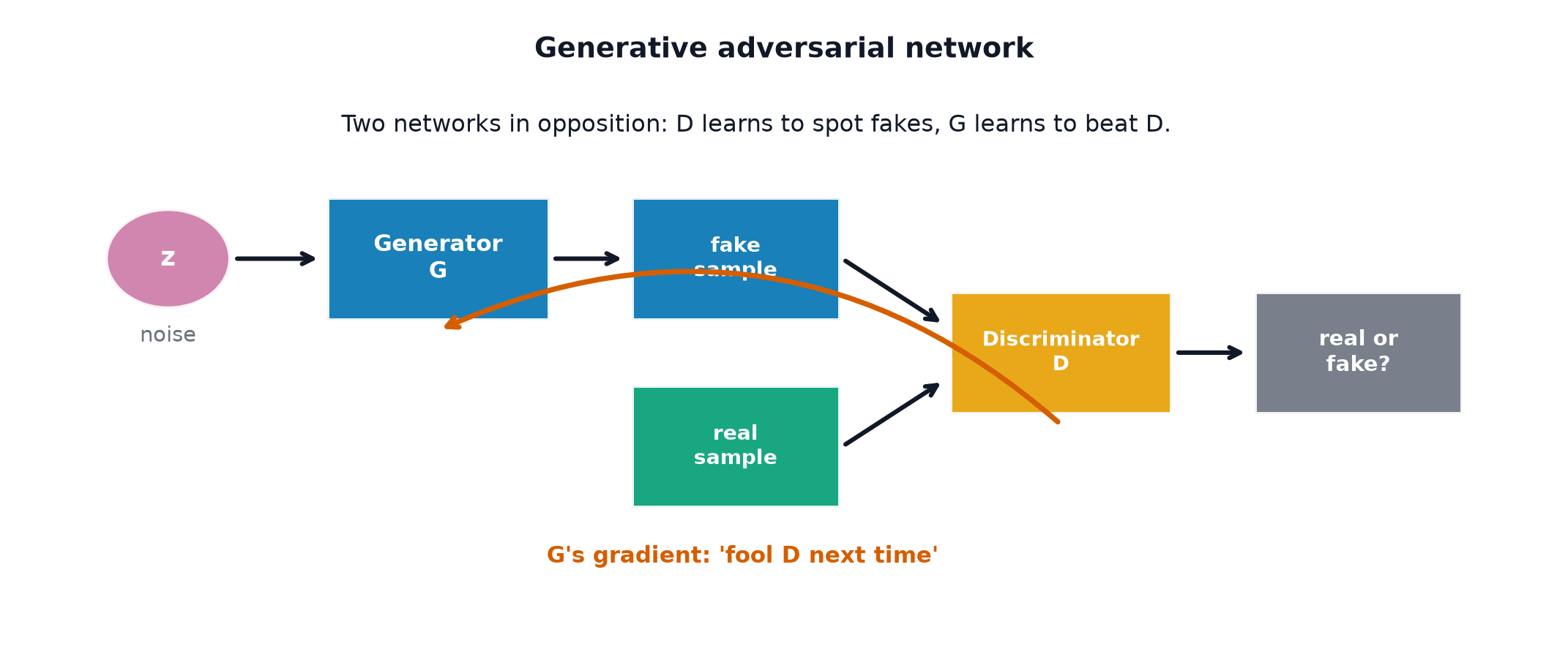
The two-player setup

A generator $G$ and a discriminator $D$ are trained simultaneously, in opposition — $G$ tries to produce samples $D$ cannot distinguish from real data; $D$ tries to correctly distinguish $G$'s generated samples from real ones. Neither network is ever told directly what "realistic" means — that entire notion is learned adversarially, through the interaction.

The generator

Maps random noise $z$ (typically drawn from a simple distribution like $\mathcal{N}(0, I)$) to a generated sample $G(z)$ — no explicit density is ever computed, making GANs the canonical implicit density model from What Is a Generative Model.

The discriminator as a learned loss

$D$ outputs the probability a given input is real (as opposed to generated) — effectively a binary classifier (Logistic Regression-style), but one whose decision boundary is itself the generator's training signal, rather than a fixed, hand-designed loss function.

The minimax objective

$$\min_G \max_D \; \mathbb{E}_{x \sim p_{\text{data}}}[\log D(x)] + \mathbb{E}_{z \sim p_z}[\log(1 - D(G(z)))]$$

$D$ maximises this (correctly classify real as real, fake as fake); $G$ minimises it (fool $D$ into misclassifying fakes as real) — a genuine two-player zero-sum game, trained by alternating gradient updates to each network.

The theoretical optimum

At the game's theoretical optimum (assuming both networks have unlimited capacity and training converges), the discriminator's output settles at $D^*(x) = 0.5$ everywhere — it can no longer distinguish real from generated at all — and the generator's distribution exactly matches the true data distribution $p_{\text{data}}$. This is a beautiful theoretical result; in practice, training rarely reaches this exact equilibrium (see GAN Training Challenges).

The non-saturating generator loss

Early in training, when the generator is still weak, $D$ can distinguish fakes easily, and $\log(1 - D(G(z)))$'s gradient becomes very small (saturated) exactly when the generator most needs a strong learning signal. The standard fix: train the generator to instead maximise $\log D(G(z))$ directly — the same fixed point, but with much stronger gradients early in training when they matter most.

Symbol	Meaning
$G, D$	the generator and discriminator networks
$z$	random noise input to the generator
$p_{\text{data}}, p_z$	the true data distribution and the noise prior

The training loop, step by step

1. Sample real data and generate fake data from noise.
2. Update $D$ to better distinguish real from fake (one or more steps).
3. Update $G$ to better fool the (now-updated) $D$.
4. Repeat.

DCGAN as the architecture that made it work

Early GANs on fully-connected networks were notoriously unstable. DCGAN specified a set of convolutional architecture and training conventions (strided convolutions instead of pooling, batch normalisation, specific activation choices) that dramatically improved GAN training stability in practice — establishing the architectural template most subsequent image GANs built on.

Conditional GANs

Feed a class label (or other conditioning information) to both the generator and discriminator — the generator learns to produce samples of a specific requested class, and the discriminator learns to check both realism and label-consistency together.

Image-to-image translation and CycleGAN, briefly

Rather than generating from pure noise, image-to-image GANs transform one image into another domain (sketches to photos, horses to zebras). CycleGAN specifically handles the case with no paired training examples available (no ground-truth "this exact sketch corresponds to this exact photo"), using a cycle-consistency constraint (translating there and back should approximately recover the original) instead.

Why GAN samples are sharp where VAE samples are blurry

Variational Autoencoders's reconstruction loss, minimised in expectation over an uncertain target, is minimised by an average — producing blur. GANs have no such pixel-wise reconstruction term at all; the discriminator only judges overall realism, with no pressure toward any particular averaging behaviour, which is a large part of why GAN samples tend to look visually sharper.

What GANs cannot give you

No likelihood (implicit density only, so no principled way to evaluate "how probable is this sample under the model"), and no reliable coverage guarantee (a GAN can achieve excellent sample quality while still failing to represent the full diversity of the true data distribution — the mode collapse failure covered fully in GAN Training Challenges).

Code: a small GAN on a 2-D ring of Gaussians, training dynamics visible

gan_demo.py

import torch
import torch.nn as nn
import matplotlib.pyplot as plt
import numpy as np

def sample_ring(n, rng):
    angles = rng.uniform(0, 2 * np.pi, n)
    radius = 3 + rng.normal(0, 0.1, n)
    return np.stack([radius * np.cos(angles), radius * np.sin(angles)], axis=1)

rng = np.random.default_rng(0)
generator = nn.Sequential(nn.Linear(2, 32), nn.ReLU(), nn.Linear(32, 32), nn.ReLU(), nn.Linear(32, 2))
discriminator = nn.Sequential(nn.Linear(2, 32), nn.ReLU(), nn.Linear(32, 32), nn.ReLU(), nn.Linear(32, 1), nn.Sigmoid())

g_optimizer = torch.optim.Adam(generator.parameters(), lr=0.001)
d_optimizer = torch.optim.Adam(discriminator.parameters(), lr=0.001)
bce = nn.BCELoss()

fig, axes = plt.subplots(1, 4, figsize=(16, 4))
snapshot_steps = [0, 500, 2000, 5000]

for step in range(5001):
    real_data = torch.tensor(sample_ring(64, rng), dtype=torch.float32)
    noise = torch.randn(64, 2)
    fake_data = generator(noise)

    d_optimizer.zero_grad()
    d_loss = bce(discriminator(real_data), torch.ones(64, 1)) + \
              bce(discriminator(fake_data.detach()), torch.zeros(64, 1))
    d_loss.backward(); d_optimizer.step()

    g_optimizer.zero_grad()
    g_loss = bce(discriminator(fake_data), torch.ones(64, 1))  # non-saturating loss
    g_loss.backward(); g_optimizer.step()

    if step in snapshot_steps:
        idx = snapshot_steps.index(step)
        with torch.no_grad():
            samples = generator(torch.randn(300, 2)).numpy()
        real_samples = sample_ring(300, rng)
        axes[idx].scatter(real_samples[:, 0], real_samples[:, 1], alpha=0.3, label="real")
        axes[idx].scatter(samples[:, 0], samples[:, 1], alpha=0.3, label="generated")
        axes[idx].set_title(f"step {step}")
        if idx == 0: axes[idx].legend()
plt.savefig("gan_training_progress.png")

See also

• GAN Training Challenges — the instability and mode collapse this page's basic recipe is prone to.
• Variational Autoencoders — the explicit-density alternative, with its own quality/coverage trade-offs.