Normalizing Flows

Every generative family so far trades away exact likelihood for something else: GANs give up density entirely, VAEs settle for a lower bound. Normalizing flows refuse that trade — by restricting every layer to be invertible, they keep an exact, computable likelihood all the way through a deep, expressive transformation.

Key idea

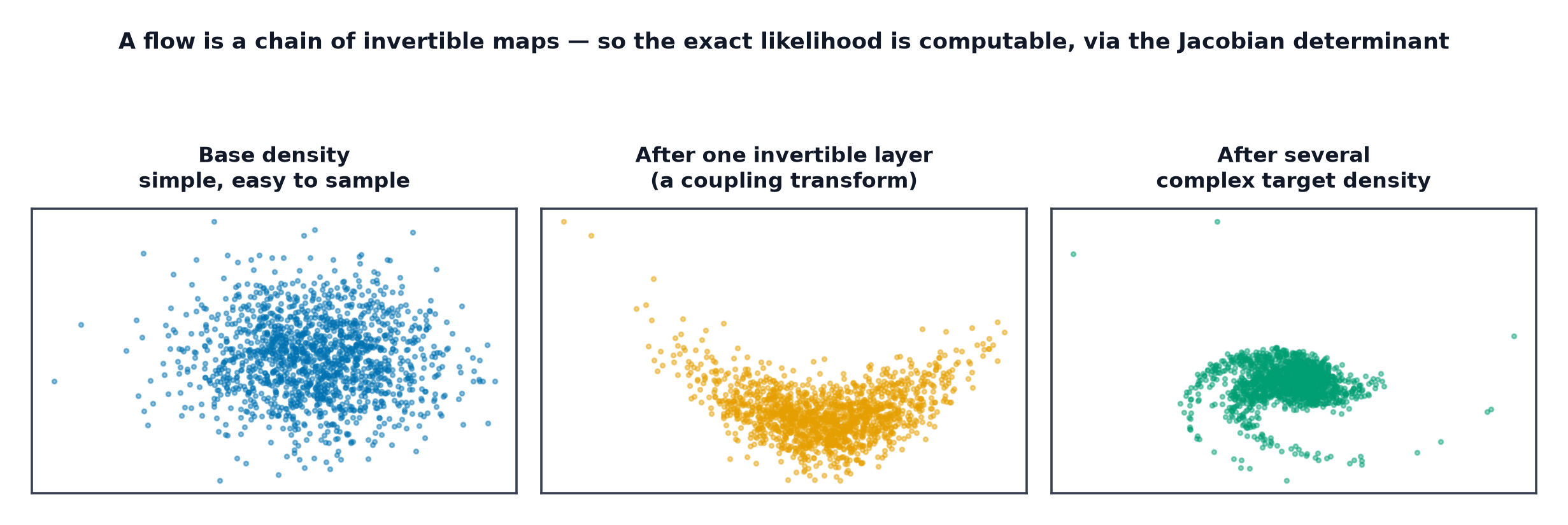
If every layer is invertible and you can compute its Jacobian determinant, you can transform a simple distribution into a complex one and still know the exact density.

A flow is a chain of *invertible* maps from a simple base density to a complex one. Invertibility is what makes the exact likelihood computable — and also what constrains the architecture severely, since every layer must have a tractable Jacobian determinant.

The change-of-variables formula for densities

If $z \sim p_z(z)$ and $x = f(z)$ for an invertible $f$, then:

$$p_x(x) = p_z(f^{-1}(x)) \left| \det \frac{\partial f^{-1}}{\partial x} \right|$$

Transforming a random variable through an invertible function changes its density by exactly the (absolute) determinant of that transformation's Jacobian — the one piece of multivariable calculus the entire flow family is built on.

Why the Jacobian determinant appears

Intuitively: the determinant measures how much a transformation locally stretches or compresses volume. A region that gets stretched has its probability mass spread thinner (lower density); a region that gets compressed has its mass concentrated (higher density). The determinant is exactly the correction factor needed to keep total probability summing to 1 after the transformation.

The two design constraints: invertibility and a tractable determinant

Any invertible neural network layer would, in principle, satisfy the change-of-variables formula — but computing a general $n \times n$ Jacobian determinant costs $O(n^3)$, prohibitive for any realistic dimensionality. Every flow architecture is a different answer to the same design question: how do you build an expressive, invertible layer whose Jacobian determinant is cheap (ideally $O(n)$) to compute?

Planar and radial flows as the simple case

The earliest flows applied simple, low-capacity invertible transformations (a single-unit "planar" perturbation, or a radial expansion/contraction around a point) whose Jacobian determinant has a closed form by construction. Individually weak, but stacking many of them composes into a genuinely expressive transformation — the same "depth over width" idea that motivates deep networks generally.

Coupling layers (RealNVP): split, transform half, keep half

Split the input $z$ into two halves, $z_a$ and $z_b$. Leave $z_a$ unchanged; transform $z_b$ using a function whose parameters are computed from $z_a$ (typically an affine scale-and-shift, output by a neural network that takes $z_a$ as input):

$$x_a = z_a, \qquad x_b = z_b \odot \exp(s(z_a)) + t(z_a)$$

Because $z_a$ passes through unchanged, the transformation is trivially invertible ($z_a = x_a$, then solve the affine equation for $z_b$ using the same $s, t$ evaluated on $x_a$), regardless of how complex $s$ and $t$ are — they never need to be inverted themselves.

Why the coupling Jacobian is triangular and therefore cheap

Because $x_a$ depends only on $z_a$, and $x_b$ depends on both, the Jacobian $\partial x / \partial z$ is block-triangular — and a triangular matrix's determinant is just the product of its diagonal entries, computable in $O(n)$ rather than $O(n^3)$. This is the single trick that makes coupling-layer flows practical at real dimensionality.

Autoregressive flows (MAF, IAF) and the sampling/density asymmetry between them

Take the coupling idea further: make each dimension's transformation depend on all previous dimensions (an autoregressive factorisation, exactly Language Modeling Basics's chain rule). MAF (Masked Autoregressive Flow) computes density fast (parallel, one pass) but samples slowly (sequential, one dimension at a time). IAF (Inverse Autoregressive Flow) has the reversed trade-off — fast parallel sampling, slow sequential density evaluation. Which one you want depends entirely on whether your use case needs fast sampling or fast likelihood.

Stacking flows with permutations between layers

A single coupling layer only transforms half the dimensions in a way that depends on the input. Alternating a permutation (or fixed shuffle) of dimensions between successive coupling layers ensures that, across the full stack, every dimension eventually gets to be in both the "unchanged" and "transformed" half — without permutation, half the dimensions would never actually interact with the transformation.

Exact likelihood as the selling point

Because every layer is invertible with a tractable Jacobian, the total log-likelihood of a flow model is exactly computable by summing the base distribution's log-density with the log-determinant of every layer — no bound, no approximation, unlike the VAE's ELBO. This makes flows directly comparable and optimisable via true maximum likelihood.

The cost: dimension-preserving layers, so no bottleneck and heavy memory

Invertibility requires that every layer map $\mathbb{R}^n \to \mathbb{R}^n$ exactly — there is no bottleneck, no dimensionality reduction anywhere in the network, unlike Autoencoders or Variational Autoencoders. This means flow models tend to be memory-heavy relative to their sample quality, and is the main practical reason flows have not displaced GANs or diffusion models for large-scale image generation.

Symbol	Meaning
$f, f^{-1}$	the flow transformation and its inverse
$z_a, z_b$	the two halves of a coupling layer's input
$s(\cdot), t(\cdot)$	the scale and shift networks in a coupling layer

Where flows are actually used

Density estimation where exact likelihood genuinely matters (scientific applications, out-of-distribution detection), as a flexible variational posterior inside other models (improving on a plain Gaussian approximate posterior), and in physics and other sciences where an exact, invertible, likelihood-computable model of a distribution is a hard requirement rather than a nice-to-have.

Code: a two-layer RealNVP-style coupling flow on two moons

normalizing_flows_demo.py

import torch
import torch.nn as nn
import matplotlib.pyplot as plt
import numpy as np

def make_two_moons(n, rng, noise=0.08):
    n1 = n // 2
    theta1 = rng.uniform(0, np.pi, n1)
    theta2 = rng.uniform(0, np.pi, n - n1)
    x1 = np.stack([np.cos(theta1), np.sin(theta1)], axis=1)
    x2 = np.stack([1 - np.cos(theta2), 1 - np.sin(theta2) - 0.5], axis=1)
    data = np.concatenate([x1, x2], axis=0)
    return data + rng.normal(0, noise, data.shape)

class CouplingLayer(nn.Module):
    def __init__(self, swap=False):
        super().__init__()
        self.swap = swap
        self.net = nn.Sequential(nn.Linear(1, 32), nn.ReLU(), nn.Linear(32, 2))

    def forward(self, z):
        za, zb = (z[:, :1], z[:, 1:]) if not self.swap else (z[:, 1:], z[:, :1])
        s, t = self.net(za).chunk(2, dim=1)
        s = torch.tanh(s)  # keep scale bounded for stability
        xb = zb * torch.exp(s) + t
        x = torch.cat([za, xb], dim=1) if not self.swap else torch.cat([xb, za], dim=1)
        log_det = s.sum(dim=1)
        return x, log_det

    def inverse(self, x):
        xa, xb = (x[:, :1], x[:, 1:]) if not self.swap else (x[:, 1:], x[:, :1])
        s, t = self.net(xa).chunk(2, dim=1)
        s = torch.tanh(s)
        zb = (xb - t) * torch.exp(-s)
        z = torch.cat([xa, zb], dim=1) if not self.swap else torch.cat([zb, xa], dim=1)
        return z

class Flow(nn.Module):
    def __init__(self):
        super().__init__()
        self.layers = nn.ModuleList([CouplingLayer(swap=False), CouplingLayer(swap=True)])

    def forward(self, z):
        log_det_total = torch.zeros(z.size(0))
        for layer in self.layers:
            z, log_det = layer(z)
            log_det_total += log_det
        return z, log_det_total

    def log_prob(self, x):
        z = x
        log_det_total = torch.zeros(x.size(0))
        for layer in reversed(self.layers):
            z_prev = layer.inverse(z)
            _, log_det = layer(z_prev)
            log_det_total += log_det
            z = z_prev
        base_log_prob = -0.5 * (z ** 2).sum(dim=1) - np.log(2 * np.pi)
        return base_log_prob - log_det_total

rng = np.random.default_rng(0)
data = torch.tensor(make_two_moons(1000, rng), dtype=torch.float32)

flow = Flow()
optimizer = torch.optim.Adam(flow.parameters(), lr=0.005)
for epoch in range(500):
    optimizer.zero_grad()
    loss = -flow.log_prob(data).mean()  # exact negative log-likelihood
    loss.backward(); optimizer.step()
    if epoch % 100 == 0:
        print(f"epoch {epoch}: exact NLL = {loss.item():.3f}")

# --- Density heatmap from the exact likelihood, and samples pushed through the flow ---
xx, yy = np.meshgrid(np.linspace(-2, 2.5, 100), np.linspace(-2, 2, 100))
grid = torch.tensor(np.stack([xx.ravel(), yy.ravel()], axis=1), dtype=torch.float32)
with torch.no_grad():
    log_density = flow.log_prob(grid).reshape(100, 100)
    samples, _ = flow(torch.randn(500, 2))

fig, axes = plt.subplots(1, 2, figsize=(10, 4))
axes[0].contourf(xx, yy, log_density.exp(), levels=30)
axes[0].set_title("exact learned density (heatmap)")
axes[1].scatter(data[:, 0], data[:, 1], alpha=0.3, label="real")
axes[1].scatter(samples[:, 0], samples[:, 1], alpha=0.3, label="flow samples")
axes[1].legend(); axes[1].set_title("samples: prior pushed through the flow")
plt.savefig("normalizing_flows_two_moons.png")

See also

• What Is a Generative Model — where flows sit in the explicit/implicit density taxonomy.
• Diffusion Models — a different route to strong density modelling, trading exact likelihood for iterative sampling.