Variational Autoencoders

Autoencoders ended on an unsolved problem: the latent space has no known structure, so there's no principled way to pick a point to decode into a new sample. The variational autoencoder's fix is direct — force the latent space to match a known distribution during training, and sampling becomes as simple as drawing from that known distribution and decoding.

Key idea

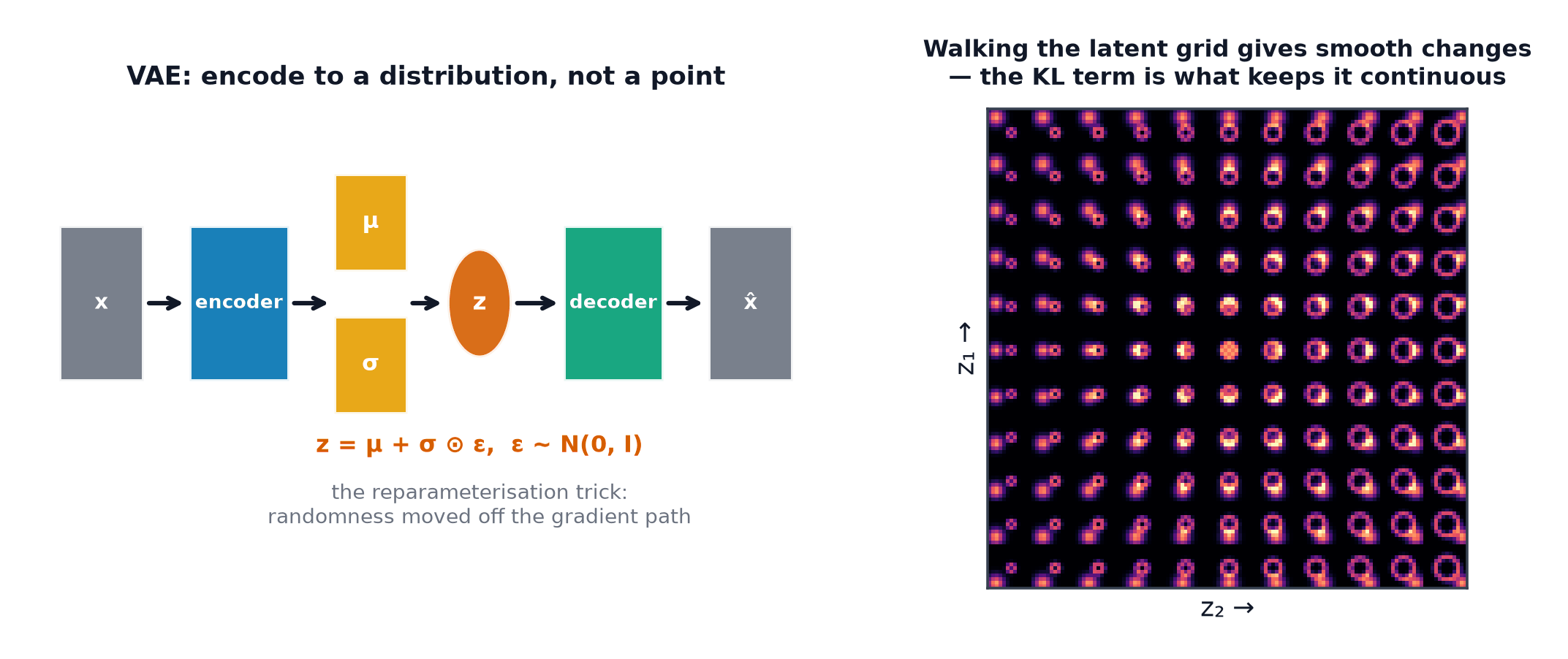
Force the latent space to match a known prior, and sampling becomes "draw from the prior and decode".

A VAE encodes to a *distribution* rather than a point, and the reparameterisation trick moves the sampling off the gradient path so backpropagation still works. The KL term is what keeps the latent space continuous enough for the grid on the right to vary smoothly.

The problem restated

A plain autoencoder's encoder maps each input to a single point in latent space, with nothing constraining the overall shape of that space — leaving gaps a random draw is likely to land in.

The probabilistic reframing

Instead of encoding to a single point, encode to a distribution — typically a Gaussian, parameterised by a mean $\mu$ and variance $\sigma^2$ that the encoder network outputs for each input. Sampling $z$ from that per-input distribution (rather than using a fixed point) injects noise that, over training, forces nearby inputs to map to overlapping regions of latent space rather than isolated points.

The prior

Additionally, constrain the aggregate distribution of all encoded points toward a fixed, known prior — typically $\mathcal{N}(0, I)$, the standard Gaussian. Once training succeeds, the latent space's overall shape is known and well-behaved by construction, not left to chance.

The ELBO, derived from the marginal likelihood

Directly maximising $\log p(x) = \log \int p(x \mid z) p(z)\, dz$ is intractable (the integral has no closed form for a useful decoder). The Evidence Lower Bound sidesteps this by introducing an approximate posterior $q(z \mid x)$ (the encoder) and optimising a tractable lower bound on the true log-likelihood instead:

$$\log p(x) \geq \mathbb{E}_{q(z|x)}[\log p(x \mid z)] - D_{KL}\big(q(z \mid x) \parallel p(z)\big) = \text{ELBO}$$

The two terms and the tension

Reconstruction term $\mathbb{E}_{q(z|x)}[\log p(x \mid z)]$: pushes the decoder to reconstruct accurately, exactly like Autoencoders's objective. KL term $D_{KL}(q(z|x) \parallel p(z))$: pushes the encoded distribution toward matching the prior. These two terms actively pull against each other — perfect reconstruction wants each input's encoding to be maximally distinctive (far from the prior, to encode maximum information), while the KL term wants every encoding pulled toward the same fixed prior. The balance between them is exactly what determines the latent space's usable structure.

Symbol	Meaning
$q(z \mid x)$	the encoder — an approximate posterior over latent $z$ given input $x$
$p(z)$	the prior over latent space, typically $\mathcal{N}(0, I)$
$p(x \mid z)$	the decoder — the likelihood of $x$ given a latent code

The reparameterisation trick

Sampling $z \sim \mathcal{N}(\mu, \sigma^2)$ directly is not differentiable with respect to $\mu, \sigma$ — you can't backpropagate through a random sampling operation. The fix: rewrite the sample as $z = \mu + \sigma \odot \epsilon$, where $\epsilon \sim \mathcal{N}(0, I)$ is sampled independently of the network's parameters — now $z$ is a deterministic, differentiable function of $\mu, \sigma$, and the randomness has been moved entirely into $\epsilon$, which needs no gradient at all.

Posterior collapse

A specific failure mode: the KL term dominates training so strongly that $q(z \mid x)$ collapses to match the prior regardless of the input — the encoder stops encoding any useful information about $x$ at all, and the decoder learns to ignore $z$ and generate a generic, input-independent output instead.

β-VAE and the disentanglement claim

Scaling the KL term by a factor $\beta > 1$ pushes harder toward matching the prior, which empirically tends to produce latent dimensions that each capture a more independent, semantically interpretable factor of variation ("disentanglement") — at a direct cost to reconstruction quality, since the stronger KL pressure competes more aggressively against the reconstruction term.

Why VAE samples are blurry

The reconstruction term is typically a Gaussian likelihood, which reduces to squared error — and squared error, minimised in expectation over an uncertain (multi-modal) target, is minimised by predicting something close to the average of the plausible outputs, not any single sharp one. This averaging effect is the standard explanation for VAE samples' characteristic blurriness relative to GAN samples.

Latent-space interpolation and arithmetic

Because the latent space is now known to be smooth and well-structured (unlike a plain autoencoder's), interpolating between two encoded points and decoding the intermediate points produces a smooth, meaningful visual transition — direct evidence the KL regularisation achieved its structural goal.

Conditional VAEs

Additionally condition both the encoder and decoder on a label or attribute $y$ — lets the model generate samples of a specific requested class, rather than an unconditional sample from the whole learned distribution.

Code: VAE on MNIST-scale data, prior sampling, latent grid, loss decomposition

vae_demo.py

import torch
import torch.nn as nn
from torchvision import datasets, transforms
import matplotlib.pyplot as plt

class VAE(nn.Module):
    def __init__(self, latent_dim=2):
        super().__init__()
        self.encoder = nn.Sequential(nn.Flatten(), nn.Linear(784, 128), nn.ReLU())
        self.mu_layer = nn.Linear(128, latent_dim)
        self.logvar_layer = nn.Linear(128, latent_dim)
        self.decoder = nn.Sequential(nn.Linear(latent_dim, 128), nn.ReLU(), nn.Linear(128, 784), nn.Sigmoid())

    def forward(self, x):
        h = self.encoder(x)
        mu, logvar = self.mu_layer(h), self.logvar_layer(h)
        std = torch.exp(0.5 * logvar)
        eps = torch.randn_like(std)
        z = mu + std * eps  # reparameterisation trick
        recon = self.decoder(z).view(-1, 1, 28, 28)
        return recon, mu, logvar

def vae_loss(recon, x, mu, logvar):
    recon_loss = nn.functional.binary_cross_entropy(recon, x, reduction="sum")
    kl_loss = -0.5 * torch.sum(1 + logvar - mu.pow(2) - logvar.exp())
    return recon_loss, kl_loss

transform = transforms.ToTensor()
train_data = datasets.MNIST(root="./data", train=True, download=True, transform=transform)
loader = torch.utils.data.DataLoader(train_data, batch_size=128, shuffle=True)

model = VAE(latent_dim=2)
optimizer = torch.optim.Adam(model.parameters(), lr=0.001)
for epoch in range(3):
    total_recon, total_kl = 0.0, 0.0
    for x, _ in loader:
        optimizer.zero_grad()
        recon, mu, logvar = model(x)
        recon_loss, kl_loss = vae_loss(recon, x, mu, logvar)
        (recon_loss + kl_loss).backward()
        optimizer.step()
        total_recon += recon_loss.item(); total_kl += kl_loss.item()
    print(f"epoch {epoch}: reconstruction={total_recon:.0f}, KL={total_kl:.0f}  (the tension, tracked separately)")

# --- Sample from the prior, and a latent grid traversal ---
fig, axes = plt.subplots(2, 8, figsize=(14, 4))
with torch.no_grad():
    for i in range(8):
        z = torch.randn(1, 2)  # sample directly from the prior
        sample = model.decoder(z).view(28, 28)
        axes[0, i].imshow(sample, cmap="gray"); axes[0, i].axis("off")
    grid_vals = torch.linspace(-2, 2, 8)
    for i, val in enumerate(grid_vals):
        z = torch.tensor([[val, 0.0]])
        traversal = model.decoder(z).view(28, 28)
        axes[1, i].imshow(traversal, cmap="gray"); axes[1, i].axis("off")
plt.savefig("vae_samples_and_traversal.png")

See also

• Autoencoders — the unstructured latent space this page's prior constraint directly fixes.
• Information Theory — the KL divergence used in the ELBO's regularisation term.