What Is a Generative Model

Every model in the classical ML and deep learning sections so far predicts a label or value from an input. A generative model asks a different, harder question: can you produce a new example that looks like it came from the same distribution as the training data? Answering "yes" requires learning something classifiers never need — an actual model of what the data looks like.

Key idea

A discriminative model learns p(y | x); a generative model learns p(x), which is a much harder question and buys you sampling.

A discriminative model needs only the boundary; a generative model learns the whole distribution. That is more work and more error-prone — but it is what makes sampling new data possible at all.

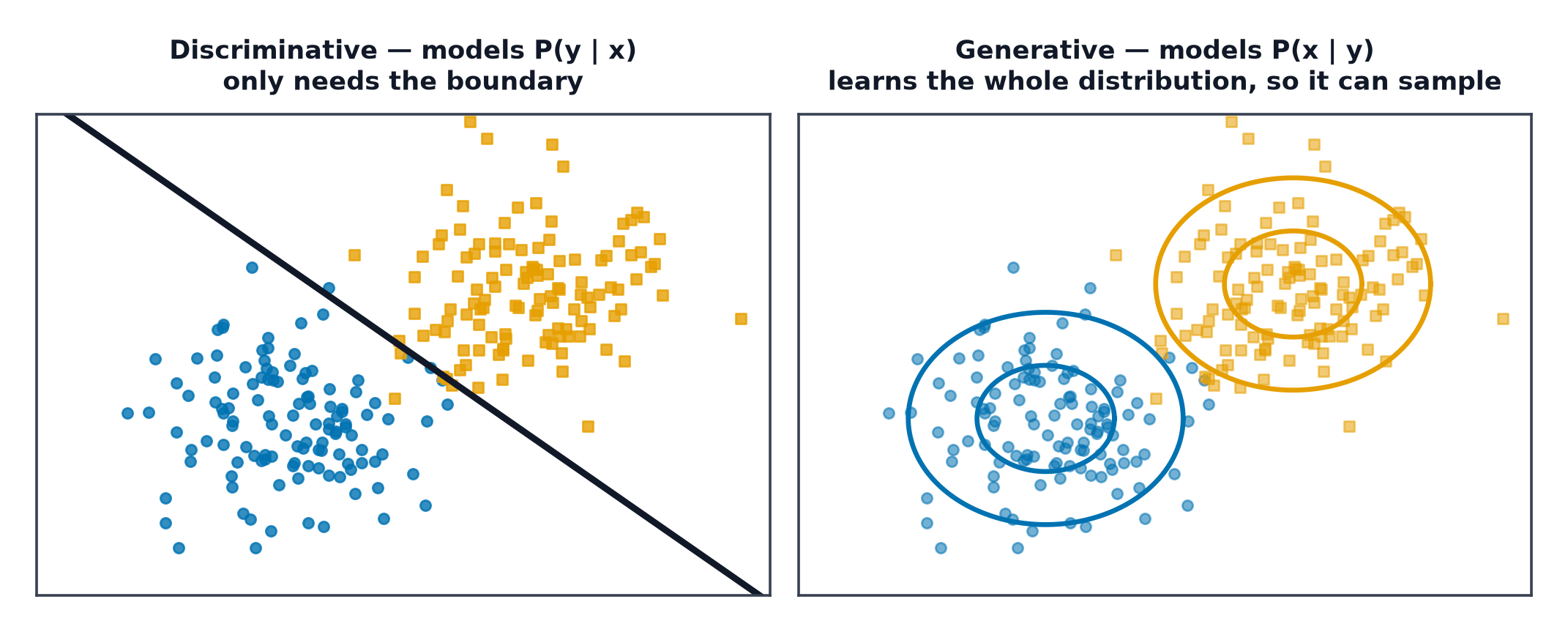
Discriminative vs. generative, stated precisely

A discriminative model learns $p(y \mid x)$ — given an input, what's the distribution over labels (Logistic Regression, most of classical ML and deep learning). A generative model learns $p(x)$ (or $p(x, y)$) — the distribution over the data itself, which is what lets you sample new, novel $x$ values, something a discriminative model has no mechanism to do at all.

What "learning a distribution" means from only samples

You never observe $p(x)$ directly — only a finite set of samples drawn from it. Every method in this section is a different strategy for approximating the true, unknown generating distribution using only that finite sample, then sampling new points from the approximation.

Explicit vs. implicit density models

Explicit density: the model can compute $p(x)$ for a given $x$ directly (autoregressive models, Normalizing Flows). Implicit density: the model can sample from $p(x)$ without ever computing an actual probability value (Generative Adversarial Networks) — a real, consequential distinction, since explicit-density models support likelihood-based evaluation and implicit-density models generally don't.

Tractable vs. approximate vs. implicit density

Tractable: exact likelihood computable directly (autoregressive models — Language Modeling Basics's chain-rule factorisation is exactly this; Normalizing Flows). Approximate: likelihood only computable as a bound, not exactly (Variational Autoencoders's ELBO). Implicit: no likelihood at all, sampling only (GANs).

The taxonomy as a decision table

Family	Density	Sampling
Autoregressive	exact	slow (sequential)
Normalizing flows	exact	fast
VAE	approximate (a bound)	fast
GAN	none (implicit)	fast
Diffusion	approximate	slow (iterative), improving

Likelihood as an objective, where it succeeds and fails

Maximum likelihood (Statistics and Estimation) is the natural training objective wherever density is tractable or approximable — it directly rewards assigning high probability to real training data. Where it fails: likelihood doesn't always correlate cleanly with perceived sample quality — a model can achieve excellent likelihood while producing samples that look worse to a human than a lower-likelihood model's samples, since likelihood rewards covering the whole data distribution (including its less "impressive" corners) rather than only producing the most visually convincing examples.

Symbol	Meaning
$p(x)$	the true, unknown data-generating distribution
$p_\theta(x)$	the model's approximation, parameterised by $\theta$

The three-way trade: quality, coverage, speed

The generative trilemma: high sample quality, broad mode coverage, and fast sampling — pick two. Diffusion buys quality and coverage with slow iterative sampling; GANs are fast and sharp but drop modes.

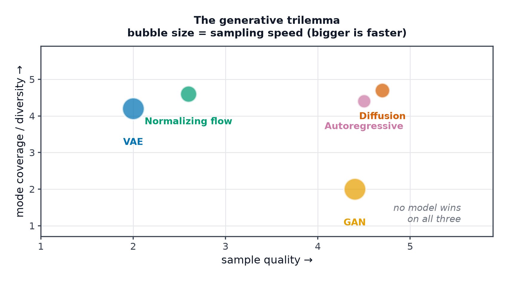
Sample quality: how convincing individual generated samples look. Mode coverage: whether the model captures the full diversity of the true distribution, or collapses onto only some of it. Sampling speed: how many computational steps are needed to produce one sample. No family in this section wins on all three simultaneously — GANs historically won quality but risked poor coverage (GAN Training Challenges); VAEs had good coverage but blurrier quality; diffusion models achieve strong quality and coverage at the cost of slow, iterative sampling (Diffusion Models, Flow Matching and Consistency Models address the speed side directly).

What generative models are used for beyond images

Data augmentation (synthesising additional training examples), anomaly detection (a point the model assigns very low likelihood to is, by that measure, anomalous — connecting directly to Anomaly Detection), compression (a good density model is, information-theoretically, an efficient code — see Information Theory), and every large language model, which is itself a generative model over token sequences.

Code: fitting a 1-D density three ways, sampling from each

what_is_generative_demo.py

import numpy as np
import matplotlib.pyplot as plt
from scipy.stats import gaussian_kde, norm

rng = np.random.default_rng(0)
true_samples = np.concatenate([rng.normal(-2, 0.5, 300), rng.normal(2, 0.8, 300)])  # bimodal

# --- Histogram density estimate ---
hist_counts, bin_edges = np.histogram(true_samples, bins=30, density=True)
def sample_from_histogram(n, rng):
    bin_idx = rng.choice(len(hist_counts), size=n, p=hist_counts / hist_counts.sum())
    return bin_edges[bin_idx] + rng.uniform(0, bin_edges[1] - bin_edges[0], size=n)

# --- KDE density estimate ---
kde = gaussian_kde(true_samples)
def sample_from_kde(n, rng):
    idx = rng.integers(0, len(true_samples), size=n)
    return true_samples[idx] + rng.normal(0, kde.factor, size=n)

# --- A small explicit parametric model: single Gaussian (deliberately too simple) ---
mu, sigma = true_samples.mean(), true_samples.std()

fig, axes = plt.subplots(1, 4, figsize=(16, 3))
axes[0].hist(true_samples, bins=30, density=True); axes[0].set_title("true distribution")
axes[1].hist(sample_from_histogram(1000, rng), bins=30, density=True); axes[1].set_title("histogram model")
axes[2].hist(sample_from_kde(1000, rng), bins=30, density=True); axes[2].set_title("KDE model")
axes[3].hist(rng.normal(mu, sigma, 1000), bins=30, density=True); axes[3].set_title("single-Gaussian (too simple)")
plt.savefig("density_models_comparison.png")

print(f"true distribution is bimodal; single-Gaussian model (mu={mu:.2f}, sigma={sigma:.2f}) cannot represent this")
print("-> exactly the taxonomy point: model family determines what distributions are even representable")

See also

• Autoencoders — the first concrete architecture this section builds toward sampling.
• Language Modeling Basics — the autoregressive, tractable-density family in its most widely-used form.