Global Methods

Global methods describe how a model behaves across the whole dataset: which features it relies on, and what shape each relationship takes.

Key idea

Permutation importance measures how much the model's score drops when a feature is scrambled — it answers "does the model rely on this?". Partial dependence shows the shape of a feature's average effect. Both are averages, and averages hide subgroups.

Global importance ranks features for the model as a whole and is unsigned — it says a feature matters, not which way it pushes. A local explanation is signed and applies to exactly one row. Neither substitutes for the other.

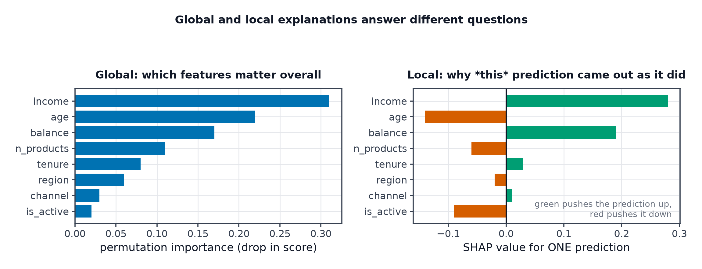
Feature importance, three ways

Method	Measures	Watch out for
Impurity / gain (trees)	Total split-criterion improvement	Biased toward high-cardinality and continuous features
Permutation	Score drop when the feature is shuffled	Misleading with correlated features; needs a held-out set
SHAP (global)	Mean absolute SHAP across rows	Slow; consistent and additive

Do not use sklearn's feature_importances_ for conclusions

The built-in impurity-based importance on tree models is systematically biased: a feature with many distinct values gets more opportunities to be split on, and accumulates spurious importance. Add a column of pure random noise with high cardinality and it will often outrank real signal.

It also uses training data, so it rewards features the model overfitted to. Use permutation importance on a held-out set, or SHAP.

Permutation importance, properly

1. Score the model on held-out data → baseline.
2. Shuffle one column, breaking its relationship with the target while preserving its marginal distribution.
3. Re-score. The drop is that feature's importance.
4. Repeat several times and average — a single shuffle is noisy.

Two properties are easy to forget. It must be computed on held-out data, or you are measuring memorisation. And with correlated features it understates importance: shuffle one of two duplicated columns and the model simply reads the other, so both look unimportant while the information is essential. Group correlated features and permute the group together.

Partial dependence and ICE

The danger of averages. The partial dependence curve on the left suggests a clean increasing effect; the ICE curves on the right reveal two subgroups moving in opposite directions. The PD curve is their average, and describes neither group.

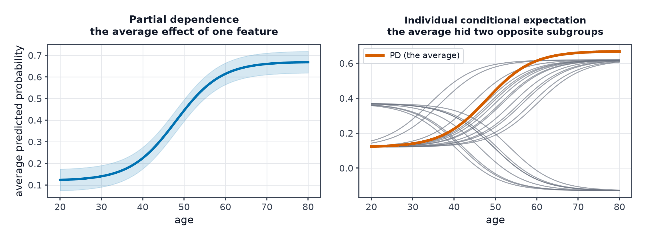
Partial dependence (PDP) answers: as feature $x_j$ varies, what happens to the average prediction? It is computed by setting $x_j$ to a value for every row, predicting, and averaging — then repeating across the feature's range.

ICE (Individual Conditional Expectation) does the same without averaging: one line per row. This is the diagnostic that catches interaction effects, because opposing subgroup effects cancel in a PDP and are invisible.

Always plot ICE alongside PDP. It costs nothing extra — the per-row predictions are already computed to make the PDP — and it is the only way to know whether the average is representative.

PDP extrapolates into impossible data

Computing partial dependence sets a feature to values while holding all others fixed, which creates rows that could not exist: a 25-year-old with 40 years of work experience, a house of 20 m² with 8 bedrooms. The model is queried far outside its training distribution, where its behaviour is arbitrary.

ALE (Accumulated Local Effects) plots fix this by averaging local changes within small windows of the feature's actual distribution. Prefer ALE when features are strongly correlated.

Surrogate models

Fit an interpretable model — a shallow tree, a linear model — to the predictions of the black box. If it reproduces them well ($R^2$ high), the surrogate is a readable approximation.

The caveat is the whole story: a surrogate with $R^2 = 0.8$ disagrees with the real model 20 % of the time, and you have no way to know which 20 %. Always report the fidelity score alongside the surrogate, and never present a low-fidelity surrogate as an explanation.

Code: permutation importance and PDP/ICE from scratch

global_methods.py

import numpy as np


def permutation_importance(predict, X, y, score_fn, n_repeats=10, seed=0):
    """Drop in score when each column is independently shuffled.

    `X` must be held-out data — computing this on training data measures
    memorisation, not reliance.
    """
    rng = np.random.default_rng(seed)
    baseline = score_fn(y, predict(X))

    means, stds = np.zeros(X.shape[1]), np.zeros(X.shape[1])
    for j in range(X.shape[1]):
        drops = []
        for _ in range(n_repeats):
            Xp = X.copy()
            rng.shuffle(Xp[:, j])                    # breaks only this column
            drops.append(baseline - score_fn(y, predict(Xp)))
        means[j], stds[j] = np.mean(drops), np.std(drops)
    return means, stds


def partial_dependence(predict, X, feature, grid_size=25):
    """PD curve plus the underlying ICE curves."""
    lo, hi = np.percentile(X[:, feature], [5, 95])    # trim tails
    grid = np.linspace(lo, hi, grid_size)

    ice = np.zeros((len(X), grid_size))
    for g, value in enumerate(grid):
        Xg = X.copy()
        Xg[:, feature] = value                       # counterfactual for EVERY row
        ice[:, g] = predict(Xg)
    return grid, ice.mean(axis=0), ice


if __name__ == "__main__":
    rng = np.random.default_rng(0)
    n = 3000
    # x0 drives y strongly, x1 weakly, x2 is pure noise, x3 duplicates x0.
    x0 = rng.normal(size=n)
    x1 = rng.normal(size=n)
    x2 = rng.normal(size=n)
    x3 = x0 + rng.normal(0, 0.05, n)                 # near-duplicate of x0
    X = np.column_stack([x0, x1, x2, x3])
    y = 3.0 * x0 + 0.6 * x1 + rng.normal(0, 0.5, n)

    split = 2000
    Xtr, Xte, ytr, yte = X[:split], X[split:], y[:split], y[split:]
    Xd = np.column_stack([np.ones(len(Xtr)), Xtr])
    coefs, *_ = np.linalg.lstsq(Xd, ytr, rcond=None)
    predict = lambda A: np.column_stack([np.ones(len(A)), A]) @ coefs
    r2 = lambda a, p: 1 - ((a - p) ** 2).sum() / ((a - a.mean()) ** 2).sum()

    imp, sd = permutation_importance(predict, Xte, yte, r2)
    for j, name in enumerate(["x0 (strong)", "x1 (weak)", "x2 (noise)", "x3 (copy of x0)"]):
        print(f"{name:>18}: {imp[j]:+.4f} ± {sd[j]:.4f}")

    print("\nNote x0 and x3 BOTH look unimportant despite carrying all the signal —")
    print("shuffle one and the model reads the other. That is the correlation trap.")

    grid, pd_curve, ice = partial_dependence(predict, Xte, feature=0)
    print(f"\nPD over x0 rises from {pd_curve[0]:+.2f} to {pd_curve[-1]:+.2f}")
    print(f"ICE spread at the midpoint: {ice[:, len(grid)//2].std():.2f}")

The output makes the correlation trap concrete: x0 and x3 between them carry all the signal, yet permutation importance rates both near zero, because destroying either leaves the other intact.

See also

• Local Methods — explaining one prediction rather than the average.
• Pitfalls and Honest Practice — where these methods break down.
• Decision Trees — the source of the biased impurity importance.