Inference Optimization

Making the model cheap enough to serve, without quietly making it wrong. Every optimisation technique on this page trades accuracy, latency, or memory for one another — measure all three, before and after, or the "optimisation" is a guess.

Key idea

Every optimisation trades accuracy, latency, or memory - measure all three before and after, or you are guessing.

Batching amortises fixed per-call overhead, so throughput climbs — but every request now waits for the whole batch. The SLA sets the ceiling, and that is what picks the batch size.

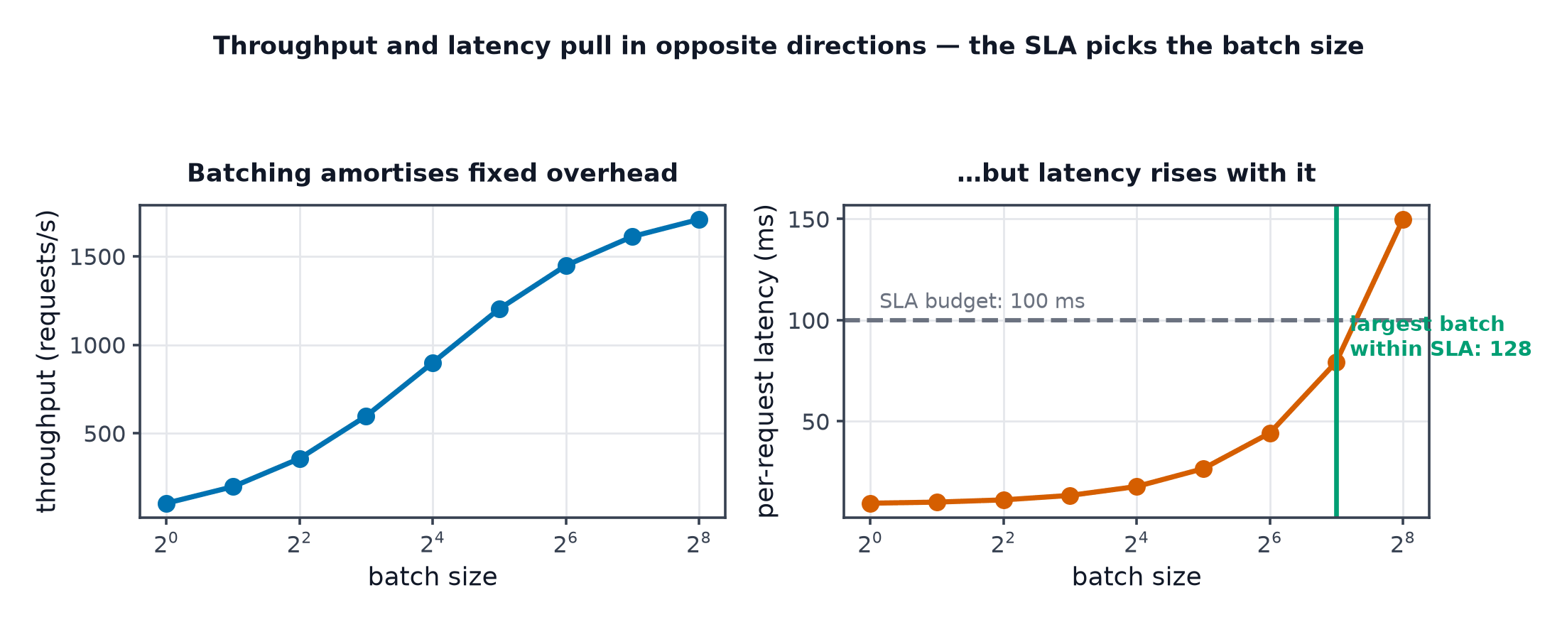
Profile before optimising: where the time actually goes

Before applying any technique below, measure where time is actually spent — preprocessing, the forward pass itself, postprocessing, or I/O. Optimising the model's forward pass when the real bottleneck is preprocessing (exactly Deploying Vision Models's latency-budget lesson) wastes effort on the part that was never the constraint.

Quantisation: dynamic, static, and quantisation-aware training

Quantization is mostly a memory and bandwidth win. Quality holds remarkably well down to INT8; below that the drop becomes real, and INT4 needs careful per-channel schemes to stay usable.

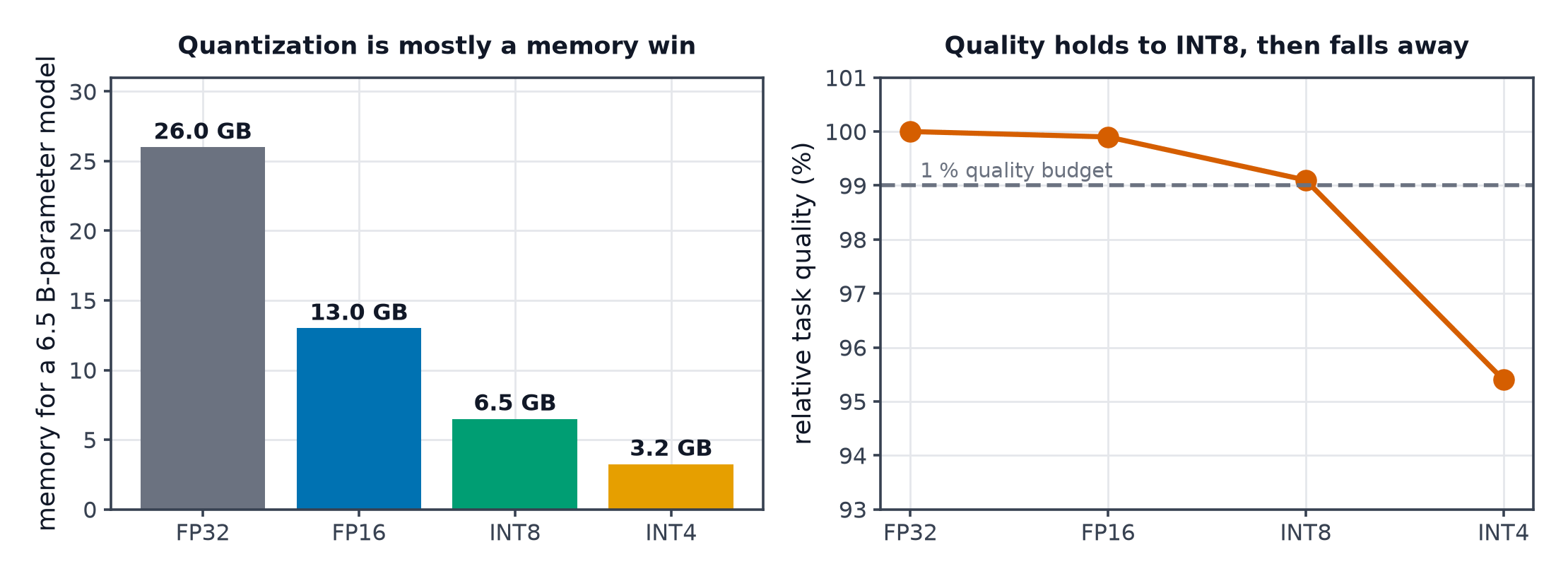
As introduced in Deploying Vision Models: dynamic quantisation converts weights at load time, activations computed at the original precision at runtime. Static quantisation quantises both ahead of time using a calibration dataset. Quantisation-aware training (QAT) simulates quantisation during training, letting the model adapt — generally the smallest accuracy cost, at the highest implementation effort.

int8 and 4-bit, and where quality drops

int8 quantisation (8-bit integers, versus 32-bit floats) typically preserves accuracy well for most models. Pushing further to 4-bit saves substantially more memory and often more latency, but quality degradation becomes noticeably more model- and task-dependent — some architectures and tasks tolerate 4-bit gracefully, others show a sharp accuracy cliff, making empirical measurement on the actual target task non-negotiable rather than something to assume from a general rule.

Pruning: structured vs. unstructured, and why unstructured rarely helps latency

Structured pruning: remove entire channels or filters — translates to real speedups on standard hardware, since the resulting computation is genuinely smaller and dense. Unstructured pruning: remove individual weights anywhere in the network — can achieve high "sparsity" numbers on paper, but without specialised sparse-computation hardware or kernels, the underlying dense matrix multiplication still runs at its original size, so latency often doesn't actually improve despite the sparsity.

Knowledge distillation: teacher, student, and the soft-target loss

Train a smaller student model to mimic a larger, already-trained teacher model's output distribution (its full probability distribution over classes, not just the hard predicted label) — the soft targets carry more information than a single correct label (relative confidence across all classes), which is why distillation typically outperforms training the same small model directly on hard labels alone.

$$L_{\text{distill}} = (1-\alpha) \, L_{\text{hard}}(y, \hat y) + \alpha \, T^2 \, L_{\text{soft}}\big(\sigma(z_{\text{teacher}}/T),\ \sigma(z_{\text{student}}/T)\big)$$

The temperature $T$ softens both distributions before comparison — a higher temperature reveals more of the teacher's relative confidence across all classes, not just its single top prediction.

Operator fusion and graph optimisation

Combining several sequential low-level operations (a matrix multiply followed by a bias add followed by an activation) into a single fused kernel reduces the overhead of launching each operation separately and the memory traffic of writing/reading intermediate results — a compiler-level optimisation orthogonal to (and stackable with) quantisation and pruning.

Compilation: TorchScript, ONNX Runtime, and vendor runtimes

Compiling a model ahead of time — via TorchScript, exporting to ONNX and running it through ONNX Runtime, or a vendor-specific runtime (targeting specific hardware) — applies graph-level optimisations automatically and produces a deployment artefact decoupled from the full training framework, both directly relevant to Model Registry and Packaging's serialisation-format choices.

KV caching and continuous batching for LLM serving

KV caching: an autoregressive language model recomputing every previous token's key/value attention state at each new generation step is wasteful — caching them avoids that redundant recomputation, a standard and essentially mandatory optimisation for LLM serving specifically. Continuous batching: rather than a rigid, fixed-size batch waiting for every sequence to finish, dynamically add new requests and remove completed ones from an in-flight batch — substantially improving GPU utilisation for variable-length generation.

Hardware-aware choices

The best optimisation strategy depends on the actual target hardware — a technique that helps on one GPU architecture (or on CPU) can be neutral or even counter-productive on another, since different hardware has different native support for lower-precision arithmetic and different memory bandwidth characteristics. Benchmarking on the actual deployment hardware, not a development machine, is what makes optimisation decisions trustworthy.

The measurement protocol

Latency percentiles, not means: p50/p95/p99 latency (the 50th/95th/99th percentile response time) reveal tail behaviour a mean can hide entirely — a mean can look fine while 1% of requests are unacceptably slow. Throughput under load: measured with realistic concurrent request volume, not single-request latency alone. Accuracy on the golden set: Offline Evaluation's evaluation suite, re-run after every optimisation to confirm quality wasn't silently traded away.

$$p_{50}, p_{95}, p_{99} = \text{the latency values below which 50\%, 95\%, 99\% of requests fall}$$

An optimisation order that avoids wasted work

1. Profile first — confirm the actual bottleneck.
2. Compile/fuse — usually free accuracy cost, apply first.
3. Quantise (dynamic, then static/QAT if needed) — measure accuracy impact at each step.
4. Distil, only if a genuinely smaller model is needed and quantisation alone isn't enough.
5. Prune, generally last, and only with structured pruning unless sparse-hardware support exists.

Symbol	Meaning
$T$	the distillation temperature
$p_{50}, p_{95}, p_{99}$	latency percentiles

Code: a baseline model measured, then quantised, with a comparison table and distillation

inference_optimization_demo.py

import torch
import torch.nn as nn
import time
import numpy as np

class TeacherModel(nn.Module):
    def __init__(self):
        super().__init__()
        self.net = nn.Sequential(nn.Linear(20, 256), nn.ReLU(), nn.Linear(256, 256), nn.ReLU(), nn.Linear(256, 10))
    def forward(self, x):
        return self.net(x)

class StudentModel(nn.Module):
    def __init__(self):
        super().__init__()
        self.net = nn.Sequential(nn.Linear(20, 32), nn.ReLU(), nn.Linear(32, 10))
    def forward(self, x):
        return self.net(x)

def measure(model, x, n_runs=100):
    with torch.no_grad():
        latencies = []
        for _ in range(n_runs):
            start = time.perf_counter()
            model(x)
            latencies.append((time.perf_counter() - start) * 1000)
    return np.percentile(latencies, 50), np.percentile(latencies, 95), np.percentile(latencies, 99)

teacher = TeacherModel().eval()
x_sample = torch.randn(1, 20)

p50, p95, p99 = measure(teacher, x_sample)
print(f"baseline (fp32):    p50={p50:.3f}ms p95={p95:.3f}ms p99={p99:.3f}ms, "
      f"size={sum(p.numel() for p in teacher.parameters())*4/1024:.1f}KB")

# --- Dynamic quantisation: re-measure latency and size ---
quantized = torch.quantization.quantize_dynamic(teacher, {nn.Linear}, dtype=torch.qint8)
p50_q, p95_q, p99_q = measure(quantized, x_sample)
print(f"quantized (int8):   p50={p50_q:.3f}ms p95={p95_q:.3f}ms p99={p99_q:.3f}ms")

with torch.no_grad():
    diff = (teacher(x_sample) - quantized(x_sample)).abs().max().item()
print(f"max output difference from quantisation: {diff:.4f}")

# --- Knowledge distillation: soft-target loss training a much smaller student ---
student = StudentModel()
optimizer = torch.optim.Adam(student.parameters(), lr=0.001)
temperature, alpha = 3.0, 0.7
X_train = torch.randn(200, 20)
y_train = torch.randint(0, 10, (200,))

for epoch in range(20):
    with torch.no_grad():
        teacher_logits = teacher(X_train)
    student_logits = student(X_train)

    hard_loss = nn.functional.cross_entropy(student_logits, y_train)
    soft_loss = nn.functional.kl_div(
        nn.functional.log_softmax(student_logits / temperature, dim=1),
        nn.functional.softmax(teacher_logits / temperature, dim=1),
        reduction="batchmean",
    ) * (temperature ** 2)
    loss = (1 - alpha) * hard_loss + alpha * soft_loss

    optimizer.zero_grad(); loss.backward(); optimizer.step()

print(f"\ndistilled student size: {sum(p.numel() for p in student.parameters())*4/1024:.1f}KB "
      f"(vs teacher's {sum(p.numel() for p in teacher.parameters())*4/1024:.1f}KB)")

See also

• Serving Patterns — the latency budget these optimisations are applied against.
• Deploying Vision Models — the same quantisation and export techniques, applied specifically to vision models.