Collaborative Filtering

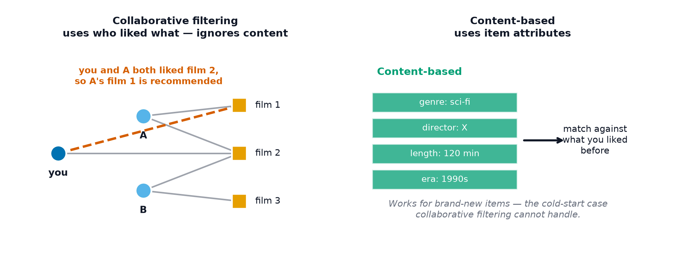
Collaborative filtering makes recommendations from interaction patterns alone. It never looks at what an item is — only at who engaged with it. That is simultaneously its great strength and the source of its cold-start failure.

Key idea

"People similar to you liked this." Neighbourhood methods compute similarity directly; matrix factorisation learns a small set of latent factors per user and per item whose dot product reconstructs the observed interactions. Both use only the interaction matrix.

Collaborative filtering routes recommendations through other users' behaviour and never inspects the item. Content-based filtering does the opposite. Their failure modes are complementary, which is why production systems hybridise them.

Neighbourhood methods

User-based: find users similar to the target, recommend what they liked. Item-based: find items similar to those the user liked, where "similar" means co-liked by the same people.

$$\hat{r}_{ui} = \frac{\sum_{v \in N(u)} \text{sim}(u,v)\, r_{vi}}{\sum_{v \in N(u)} |\text{sim}(u,v)|}$$

	User-based	Item-based
Similarity over	Users	Items
Stability	Users change fast	Item similarity is stable
Precompute	Hard — users are many and volatile	Easy — cache the item–item matrix
Explanation	"Users like you…"	"Because you watched X"

Item-based won in practice, and Amazon's item-to-item paper is the standard reference. Two reasons: there are usually fewer items than users, and item–item similarity changes slowly enough to precompute offline and serve from a cache.

Similarity measures

Measure	Notes
Cosine	Standard; ignores rating scale
Pearson	Cosine on mean-centred ratings — corrects for users who rate everything highly
Adjusted cosine	Centres by user mean, for item–item similarity
Jaccard	For implicit binary data

Mean-centring matters more than it looks. Without it, a user who rates everything 4–5 appears similar to everyone, and a harsh rater appears similar to nobody, purely as an artefact of scale.

Matrix factorisation

Approximate the sparse matrix $R$ ($m$ users × $n$ items) as the product of two thin matrices:

$$R \approx U V^\top, \qquad U \in \mathbb{R}^{m \times k},\ V \in \mathbb{R}^{n \times k}$$

Each user and each item becomes a $k$-dimensional vector, and a predicted affinity is their dot product. With $k \approx 50$, a $10^6 \times 10^5$ matrix is represented by about $5.5 \times 10^7$ parameters instead of $10^{11}$ cells.

The latent factors are learned, not designed, and are typically not interpretable — though on film data some axes do turn out to correspond loosely to recognisable dimensions like "arthouse ↔ blockbuster".

The objective

Crucially, the sum runs only over observed entries:

$$\min_{U,V} \sum_{(u,i) \in \mathcal{K}} \left(r_{ui} - \mu - b_u - b_i - \mathbf{u}_u^\top \mathbf{v}_i\right)^2 + \lambda\left(\|\mathbf{u}_u\|^2 + \|\mathbf{v}_i\|^2 + b_u^2 + b_i^2\right)$$

The bias terms do most of the early work

$\mu + b_u + b_i$ — the global mean, plus a per-user and a per-item offset — captures "this user rates generously" and "this item is well liked overall". On the Netflix Prize data, biases alone accounted for a large share of the achievable improvement, before any interaction term.

Fit them. A factorisation without bias terms wastes latent dimensions re-learning what two scalars would have captured.

SVD is not what this is

Classical SVD requires a complete matrix and is undefined with missing entries. Filling the gaps with zeros or means before applying SVD both distorts the data and destroys the sparsity that made the problem tractable.

What the recommender literature calls "SVD" (Funk's method from the Netflix Prize) is a different algorithm: gradient descent on the observed entries only. The name is historical and misleading. See PCA and SVD for the actual decomposition.

Fitting it

Method	Notes
SGD	Simple, scales well, easy to extend with extra terms
ALS	Fix $U$, solve for $V$ exactly, alternate. Parallelises well; the default for implicit feedback
BPR	Optimises ranking directly by contrasting observed against sampled unobserved items

BPR (Bayesian Personalised Ranking) deserves emphasis: it optimises the pairwise objective "the user prefers the item they interacted with over one they did not", which is much closer to the actual task than reconstructing a rating.

Implicit feedback needs a different objective

For implicit data the matrix holds counts, not ratings, and there are no negatives. The standard treatment (Hu, Koren & Volinsky) splits each entry into a preference and a confidence:

$$p_{ui} = \begin{cases} 1 & r_{ui} > 0 \\ 0 & r_{ui} = 0 \end{cases} \qquad c_{ui} = 1 + \alpha r_{ui}$$

Every cell now enters the loss — including unobserved ones — but weighted by confidence. Unobserved cells get weight 1 (a weak signal that the user might not like it); heavily interacted cells get large weights. This is what makes the objective well-posed without inventing negatives.

Where it fails

• Cold start. No interactions, no recommendation. Structural, not fixable within CF.
• Popularity bias. Popular items appear in more co-occurrences and dominate.
• Sparsity. Users with two interactions have essentially no signal.
• Grey sheep. Users whose taste matches no cohort.
• Shilling attacks. Fake accounts can be injected to manipulate item similarity.

The first is what content-based and hybrid methods exist to solve.

Code: matrix factorisation with biases, by SGD

matrix_factorization.py

import numpy as np


class MatrixFactorization:
    """Funk-style MF with bias terms, trained by SGD on observed entries only."""

    def __init__(self, n_factors=20, lr=0.01, reg=0.05, n_epochs=40, seed=0):
        self.k, self.lr, self.reg, self.n_epochs = n_factors, lr, reg, n_epochs
        self.rng = np.random.default_rng(seed)

    def fit(self, rows, cols, vals, n_users, n_items, verbose=True):
        self.mu = vals.mean()
        self.bu = np.zeros(n_users)
        self.bi = np.zeros(n_items)
        self.U = self.rng.normal(0, 0.1, (n_users, self.k))
        self.V = self.rng.normal(0, 0.1, (n_items, self.k))

        order = np.arange(len(vals))
        for epoch in range(self.n_epochs):
            self.rng.shuffle(order)
            total = 0.0
            for idx in order:
                u, i, r = rows[idx], cols[idx], vals[idx]
                err = r - self._predict_one(u, i)
                total += err * err

                bu_old, bi_old = self.bu[u], self.bi[i]
                self.bu[u] += self.lr * (err - self.reg * bu_old)
                self.bi[i] += self.lr * (err - self.reg * bi_old)

                U_old = self.U[u].copy()
                self.U[u] += self.lr * (err * self.V[i] - self.reg * U_old)
                self.V[i] += self.lr * (err * U_old - self.reg * self.V[i])

            if verbose and epoch % 10 == 0:
                print(f"  epoch {epoch:>3}: train RMSE {np.sqrt(total / len(vals)):.4f}")
        return self

    def _predict_one(self, u, i):
        return self.mu + self.bu[u] + self.bi[i] + self.U[u] @ self.V[i]

    def predict(self, rows, cols):
        return np.array([self._predict_one(u, i) for u, i in zip(rows, cols)])

    def recommend(self, u, k=5, exclude=()):
        scores = self.mu + self.bu[u] + self.bi + self.V @ self.U[u]
        scores[list(exclude)] = -np.inf         # never re-recommend seen items
        return np.argsort(-scores)[:k]


if __name__ == "__main__":
    rng = np.random.default_rng(0)
    n_users, n_items, k_true = 300, 150, 4

    # Synthesise data that genuinely has low-rank structure plus biases.
    U_true = rng.normal(0, 0.6, (n_users, k_true))
    V_true = rng.normal(0, 0.6, (n_items, k_true))
    bu_true, bi_true = rng.normal(0, 0.3, n_users), rng.normal(0, 0.4, n_items)

    n_obs = 12_000
    rows = rng.integers(0, n_users, n_obs)
    cols = rng.integers(0, n_items, n_obs)
    vals = np.clip(3.5 + bu_true[rows] + bi_true[cols]
                   + np.sum(U_true[rows] * V_true[cols], axis=1)
                   + rng.normal(0, 0.3, n_obs), 1, 5)
    print(f"density: {n_obs / (n_users * n_items) * 100:.1f} %")

    split = int(0.85 * n_obs)
    model = MatrixFactorization(n_factors=8, n_epochs=41).fit(
        rows[:split], cols[:split], vals[:split], n_users, n_items)

    pred = np.clip(model.predict(rows[split:], cols[split:]), 1, 5)
    actual = vals[split:]
    rmse = np.sqrt(np.mean((actual - pred) ** 2))
    baseline = np.sqrt(np.mean((actual - vals[:split].mean()) ** 2))
    print(f"\ntest RMSE          {rmse:.4f}")
    print(f"global-mean baseline {baseline:.4f}")
    print(f"top-5 for user 0: {model.recommend(0, 5)}")

Comparing against the global-mean baseline is the equivalent of the naive forecast in time series: it is the number the model has to beat before its complexity is justified.

See also

• The Recommendation Problem — sparsity and feedback loops.
• Content-Based and Hybrid — solving cold start.
• PCA and SVD — the actual decomposition this method is named after but does not use.