Evaluating Recommenders

Recommender evaluation is unusually treacherous: the offline metric is computed on data generated by a previous model, the ranking metrics disagree with each other, and the correlation between offline improvement and online business impact is famously weak.

Key idea

RMSE on ratings measures the wrong thing — users see a ranked list, not a predicted number. Use ranking metrics offline, treat them as a filter rather than a verdict, and settle the decision with an online experiment.

Position matters: NDCG's logarithmic discount makes a hit at rank 1 worth roughly three times one at rank 10. On the right, the precision/recall trade as k grows — and k is fixed by how many slots the interface has, not by the model.

Why RMSE is the wrong metric

The Netflix Prize optimised RMSE on predicted ratings. It is a poor proxy for recommendation quality, for reasons that took the field some years to fully absorb:

• Users are shown a ranked list; the ordering is what they experience.
• Errors on items the user will never see are weighted equally with errors on the top slot.
• Most production data is implicit, where there is no rating to predict at all.

The famous coda: Netflix never deployed the winning ensemble. The engineering cost was not justified by the improvement, and the metric it optimised was not the one that mattered.

Ranking metrics

Metric	Measures	Notes
Precision@k	Fraction of the k shown that are relevant	Ignores order within k
Recall@k	Fraction of all relevant items captured in k	Penalises users with many relevant items
MAP@k	Mean average precision	Order-sensitive
MRR	1 / rank of the first relevant hit	For "one right answer" tasks like search
NDCG@k	Gain discounted by log position	The standard; handles graded relevance
Hit rate@k	Did any relevant item appear?	Blunt but readable

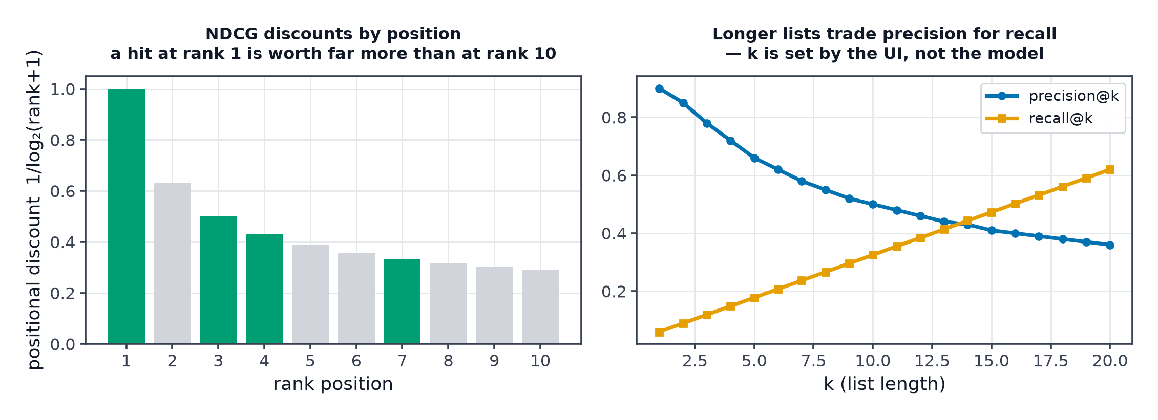
NDCG is the default because it is the only common metric that both respects position and supports graded relevance (a 5-star item counts more than a 3-star one):

$$\text{DCG@}k = \sum_{i=1}^{k} \frac{2^{rel_i} - 1}{\log_2(i + 1)}, \qquad \text{NDCG@}k = \frac{\text{DCG@}k}{\text{IDCG@}k}$$

The normalisation by the ideal DCG is what makes values comparable across users with different numbers of relevant items.

Beyond-accuracy metrics

Report these alongside accuracy, or you will ship a system that recommends the ten most popular items to everyone:

Metric	Definition
Coverage	Fraction of the catalogue appearing in anyone's top-k
Intra-list diversity	Mean pairwise dissimilarity within one list
Novelty	Mean inverse popularity of recommended items
Gini / entropy	How concentrated recommendations are across the catalogue
Serendipity	Relevant and unexpected

Splitting is not straightforward

Strategy	Description	Verdict
Random split of interactions	Shuffle all interactions	Wrong — leaks the future
Temporal / global timeline	Everything before time T trains	Most realistic
Leave-one-out	Hold out each user's most recent item	Common, mildly optimistic
User-based split	Hold out whole users	Tests cold-start generalisation

Random splitting has the same defect as in time series: it lets the model train on interactions that happened after the ones it is tested on. Reported gains routinely fail to reproduce online for exactly this reason.

Sampled metrics are not comparable

A widespread shortcut ranks the held-out positive against 100 sampled negatives instead of the whole catalogue. It is much cheaper — and it does not preserve the ranking of methods. Krichene and Rendle showed that models ranked by sampled metrics can reverse order under full-catalogue evaluation.

If you use sampling, say so, keep the sample size fixed across compared models, and never compare a sampled number against a published full-catalogue one.

Offline metrics disagree with online results

This is the field's central practical difficulty. An offline improvement in NDCG frequently produces no online lift, and occasionally a decline. The reasons are structural:

• Missing-not-at-random data. You only observe feedback on what the old model showed, so offline evaluation rewards agreeing with the old model.
• Unobserved relevance. An item the user never saw is scored as irrelevant, so genuinely good novel recommendations are punished.
• Presentation effects. Position, thumbnail, and page context drive clicks independently of the model.
• Proxy mismatch. Clicks are not satisfaction; watch time is not enjoyment; engagement is not retention.

The working conclusion: use offline metrics to filter out clearly worse candidates cheaply, and require an online experiment before believing anything.

Counterfactual / off-policy evaluation — inverse propensity scoring and its variants — partially bridges the gap by reweighting logged data by the probability the old system had of showing each item. It needs logged propensities, which means deciding to record them before you need them.

Online

Approach	Use
A/B test	The standard; randomise users, not sessions
Interleaving	Mix two rankers' results in one list — far more sensitive, needs less traffic
Bandits	Continuous allocation toward the better variant

Interleaving is under-used and worth knowing: because each user sees both rankers' output, it removes between-user variance and can detect differences with an order of magnitude less traffic than a conventional A/B test.

Guard against the metric you optimise: click-through rate rewards clickbait, so pair it with a long-horizon metric (next-week retention, completed sessions) and monitor both.

Code: NDCG, precision/recall@k, coverage and diversity

rec_metrics.py

import numpy as np


def dcg_at_k(relevances, k):
    rel = np.asarray(relevances)[:k]
    discounts = np.log2(np.arange(2, len(rel) + 2))
    return float(((2 ** rel - 1) / discounts).sum())


def ndcg_at_k(ranked_relevance, k):
    """Normalise by the best achievable ordering of the same relevances."""
    ideal = dcg_at_k(sorted(ranked_relevance, reverse=True), k)
    return dcg_at_k(ranked_relevance, k) / ideal if ideal > 0 else 0.0


def precision_recall_at_k(recommended, relevant, k):
    top = list(recommended)[:k]
    hits = len(set(top) & set(relevant))
    precision = hits / k
    recall = hits / len(relevant) if relevant else 0.0
    return precision, recall


def average_precision(recommended, relevant, k):
    hits, score = 0, 0.0
    for i, item in enumerate(list(recommended)[:k], start=1):
        if item in relevant:
            hits += 1
            score += hits / i
    return score / min(len(relevant), k) if relevant else 0.0


def catalogue_coverage(all_recommendations, n_items):
    shown = {item for rec in all_recommendations for item in rec}
    return len(shown) / n_items


def intra_list_diversity(recommended, item_vectors):
    """Mean pairwise cosine DISsimilarity within one list."""
    V = item_vectors[list(recommended)]
    V = V / np.maximum(np.linalg.norm(V, axis=1, keepdims=True), 1e-9)
    sims = V @ V.T
    n = len(V)
    if n < 2:
        return 0.0
    off_diagonal = (sims.sum() - np.trace(sims)) / (n * (n - 1))
    return 1 - off_diagonal


if __name__ == "__main__":
    rng = np.random.default_rng(0)
    n_items = 500
    item_vectors = rng.normal(size=(n_items, 16))

    relevant = {3, 17, 42, 88, 150}
    good = [3, 17, 201, 42, 9, 88, 300, 12, 150, 7]     # hits near the top
    poor = [201, 9, 300, 12, 7, 3, 17, 42, 88, 150]     # same hits, ranked low

    print(f"{'':<10}{'P@10':>8}{'R@10':>8}{'MAP@10':>9}{'NDCG@10':>10}")
    for name, rec in [("good", good), ("poor", poor)]:
        rel_vector = [1 if i in relevant else 0 for i in rec]
        p, r = precision_recall_at_k(rec, relevant, 10)
        print(f"{name:<10}{p:>8.2f}{r:>8.2f}"
              f"{average_precision(rec, relevant, 10):>9.3f}"
              f"{ndcg_at_k(rel_vector, 10):>10.3f}")

    print("\nPrecision and recall are IDENTICAL for both lists — they ignore order.")
    print("Only MAP and NDCG detect that one puts its hits at the top.\n")

    popular_everywhere = [list(range(10)) for _ in range(200)]
    personalised = [list(rng.choice(n_items, 10, replace=False)) for _ in range(200)]
    print(f"coverage, popularity-only : {catalogue_coverage(popular_everywhere, n_items):.3f}")
    print(f"coverage, personalised    : {catalogue_coverage(personalised, n_items):.3f}")
    print(f"diversity of one list     : {intra_list_diversity(personalised[0], item_vectors):.3f}")

The first block makes the central point concretely: precision@10 and recall@10 score both lists identically, because neither metric looks at order. Only MAP and NDCG distinguish a list that puts its hits in the top three from one that buries them at the bottom — which is the entire user experience.

See also

• The Recommendation Problem — feedback loops that make offline evaluation biased.
• Online Evaluation and A/B Testing — the experiment design this defers to.
• Validation and Backtesting — the same chronological-splitting discipline.