The Recommendation Problem

Recommendation looks like supervised learning and behaves nothing like it. The data is almost entirely missing, the missingness is not random, the output is a ranked list rather than a prediction, and the model's own outputs determine what data you collect next.

Key idea

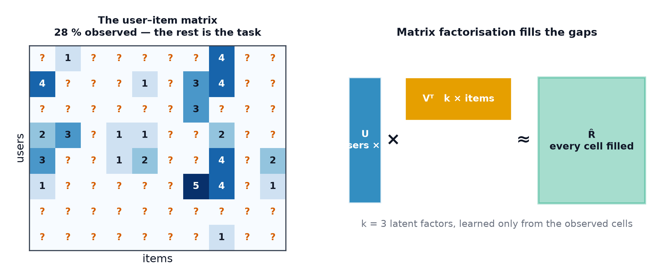
The user–item matrix is typically 99 %+ empty, and the empty cells are not missing at random — people watch what they were shown. Recommendation is a ranking problem under feedback loops, not a regression problem on ratings.

The task in one picture: most of the matrix is unobserved, and the goal is to fill it. Factorisation does that by learning a small number of latent factors per user and per item from the cells you do have.

Why it is not ordinary supervised learning

	Ordinary supervised	Recommendation
Data density	Every row has a label	99–99.9 % of cells empty
Missingness	Usually ignorable	Informative — you only rate what you saw
Output	One prediction	A ranked list of k items
Metric	Accuracy, RMSE	NDCG, recall@k, and business metrics
Feedback	Static dataset	The model shapes its own future data
New rows	Fine	Cold start — new users and items have no history

Explicit and implicit feedback

Explicit — a rating the user deliberately gave. Unambiguous but extremely rare; most users never rate anything, and those who do are unrepresentative.

Implicit — clicks, watches, purchases, dwell time. Abundant, and how essentially all production systems work. But it carries a catch:

Implicit feedback has no negatives

A user who did not click an item may have disliked it — or never seen it. Absence of interaction is not evidence of dislike, but the naive framing treats every unobserved cell as a zero.

This is why implicit-feedback models use confidence-weighted objectives (weight observed interactions highly, unobserved ones weakly) or sample negatives explicitly, rather than treating the matrix as a complete label set.

The sparsity numbers

A mid-sized service: 1 million users, 100,000 items, 50 million interactions.

$$\text{density} = \frac{5 \times 10^7}{10^6 \times 10^5} = 0.05\%$$

99.95 % of the matrix is unknown. Any method that requires the full matrix in memory is out — the matrix has $10^{11}$ cells — and any method needing dense per-user data will fail for the long tail of users with three interactions.

The two-stage architecture

No production system scores a whole catalogue per request. Cheap approximate retrieval cuts millions to hundreds; an expensive model ranks those; a final pass applies diversity and business rules. The latency budget is what forces this shape.

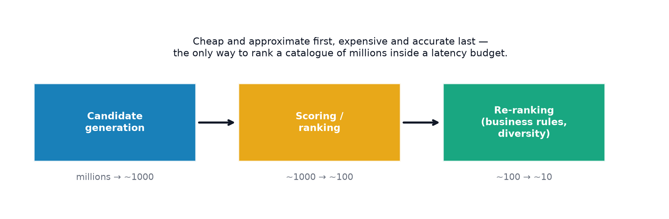
Stage	Scale	Model
Candidate generation	millions → ~1,000	Cheap: approximate nearest neighbour over embeddings, co-occurrence, popularity
Ranking	~1,000 → ~100	Expensive: gradient boosting or a deep model with rich features
Re-ranking	~100 → ~10	Diversity, freshness, business rules, de-duplication

Recall matters at stage one — an item not retrieved can never be recommended, whatever the ranker would have done with it. Precision matters at stage two.

Cold start

Case	Problem	Mitigations
New user	No history to match on	Popularity, onboarding survey, demographics, contextual bandits
New item	Nobody has interacted with it	Content features, forced exploration
New system	Neither	Content-based only until interactions accumulate

Cold start is not an edge case. On a catalogue with constant new arrivals — news, marketplaces, short video — most of the inventory is always cold, and a pure collaborative-filtering system structurally cannot surface any of it. That is the main practical argument for hybrid models.

Feedback loops

A recommender trains on data generated by its own previous recommendations. Items it showed get interactions; items it did not show get none, and so look unpopular, and so are shown even less.

The consequences compound:

• Popularity bias. Popular items are recommended more, become more popular, and crowd out the tail.
• Filter bubbles. Narrow user profiles get narrower.
• Offline metrics become self-congratulatory. A model evaluated on logged data is rewarded for agreeing with the model that produced the logs.

Mitigations are all forms of deliberate exploration: ε-greedy or bandit-based slots, inverse-propensity weighting when training on logged data, and explicit diversity terms in re-ranking. None is free — exploration costs short-term engagement to buy long-term data quality, and that trade is a product decision.

Beyond accuracy

A recommender that maximises predicted rating alone tends to be a bad product. The dimensions that matter alongside accuracy:

Property	Question
Coverage	What fraction of the catalogue ever gets recommended?
Diversity	Are the k items different from each other?
Novelty	Are they things the user would not have found alone?
Serendipity	Are they surprising and liked?
Fairness	Do item providers get equitable exposure?

Recommending the ten most popular items to everyone scores respectably on accuracy metrics and is a useless product. This is why the field moved from RMSE to ranking metrics, and then to online experiments — covered in Evaluating Recommenders.

See also

• Collaborative Filtering — the neighbourhood and factorisation methods.
• Content-Based and Hybrid — how cold start is actually handled.
• Evaluating Recommenders — ranking metrics and online tests.