Actor-Critic Methods

Policy Gradient Methods needed a full Monte Carlo return to compute a low-noise gradient — waiting for episodes to finish, and paying for it in variance. Actor-critic methods replace that Monte Carlo estimate with a second, learned network that predicts value directly, combining the direct optimisation of policy gradients with the low variance of TD learning.

Key idea

Use a learned value function as the policy gradient's baseline and you get TD's low variance with policy gradient's direct optimisation.

Where the algorithms sit relative to each other. Actor–critic methods are the middle ground this page occupies: a policy that acts, plus a value estimate that criticises, which cuts the variance that plagues pure policy gradients.

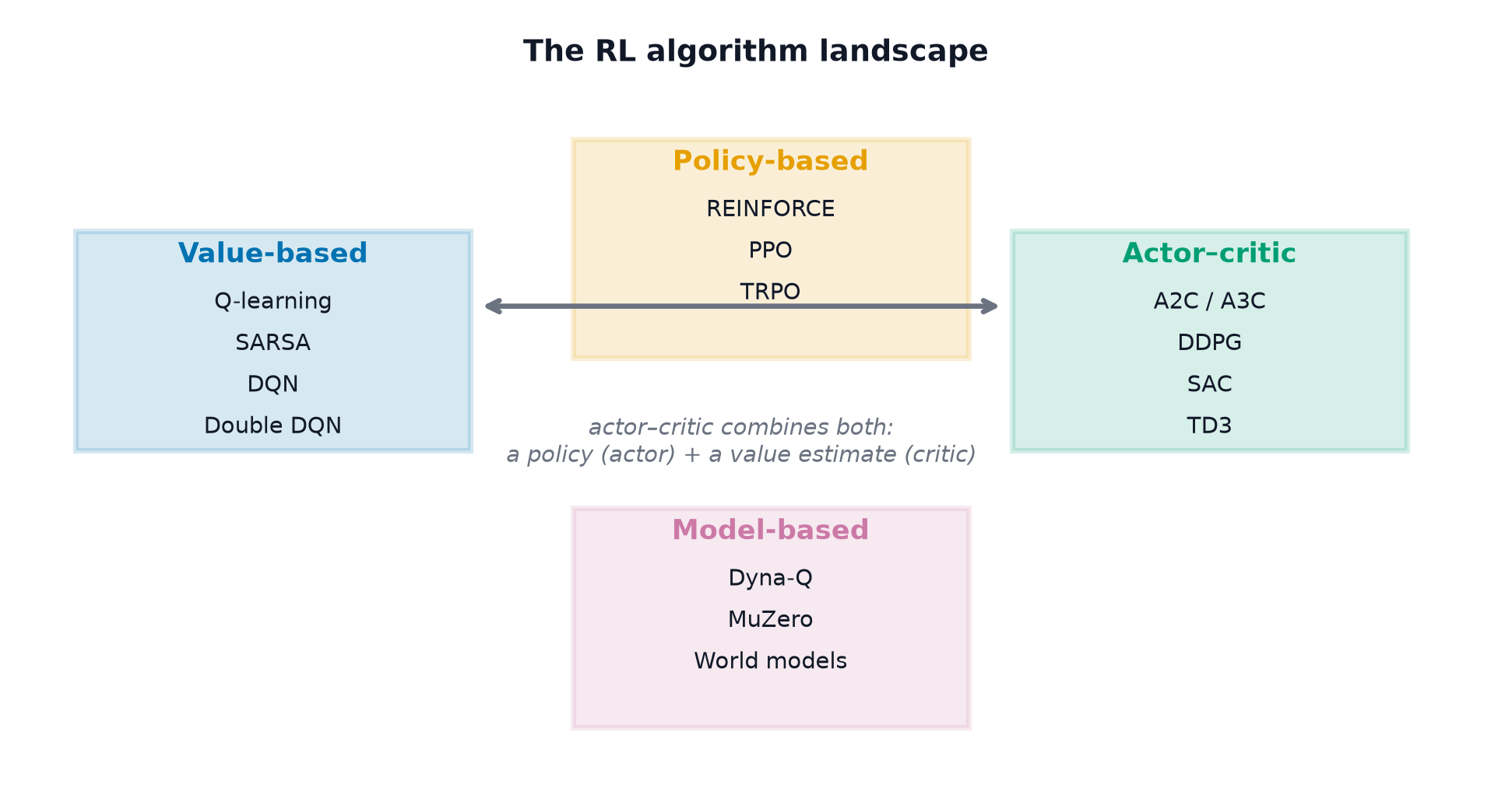
The two components: actor and critic

The actor is the policy $\pi_\theta(a \mid s)$, exactly as in Policy Gradient Methods — it selects actions. The critic is a learned value function $V_\phi(s)$ (or $Q_\phi(s,a)$), trained via TD learning (Monte Carlo and TD Learning) to estimate how good the actor's choices actually are — the critic's only job is to judge, feeding that judgement back to improve the actor.

Using the critic as the baseline

Rather than Policy Gradient Methods's Monte Carlo reward-to-go, use the critic's own learned $V_\phi(s)$ as the baseline — obtained from a single learned function, updated online every step, rather than requiring a full episode's actual returns.

The advantage actor-critic update

$$\nabla_\theta J(\theta) \approx \nabla_\theta \log \pi_\theta(a_t \mid s_t) \, \hat A_t, \qquad \hat A_t = r_{t+1} + \gamma V_\phi(s_{t+1}) - V_\phi(s_t)$$

The advantage estimate $\hat A_t$ here is exactly the TD error $\delta_t$ from Monte Carlo and TD Learning — computable after a single step, with no need to wait for an episode to end.

TD error as an unbiased estimate of the advantage

Because $\mathbb{E}[r_{t+1} + \gamma V^\pi(s_{t+1})] = Q^\pi(s_t, a_t)$ by the Bellman equation, the TD error $\delta_t = r_{t+1} + \gamma V^\pi(s_{t+1}) - V^\pi(s_t)$ is (given a correct $V^\pi$) an unbiased estimator of the true advantage $A^\pi(s_t, a_t) = Q^\pi(s_t,a_t) - V^\pi(s_t)$ — the theoretical justification for using it directly as the policy gradient's per-step signal.

The bias/variance position of actor-critic relative to REINFORCE and DQN

Actor-critic sits deliberately between two extremes: Policy Gradient Methods's REINFORCE is unbiased but high-variance (full Monte Carlo returns); using a learned, imperfect critic introduces some bias (the critic isn't exactly $V^\pi$ during training) in exchange for substantially lower variance (a single-step TD estimate rather than a whole-episode sample) — the same bias/variance trade Monte Carlo and TD Learning established for prediction, now applied inside a policy gradient.

A2C and A3C, and what parallel environments buy

A2C (Advantage Actor-Critic) runs multiple environment copies in parallel, collecting a batch of experience across all of them before each update — reduces the correlation between consecutive samples within a single trajectory, similar in spirit to Deep Q-Networks's experience replay, but achieved through parallelism rather than a stored buffer (which on-policy methods can't use directly). A3C (Asynchronous Advantage Actor-Critic) takes this further, with each parallel worker computing gradients independently and applying them asynchronously to a shared set of parameters.

Generalised advantage estimation and the λ dial

$$\hat A_t^{\text{GAE}(\lambda)} = \sum_{k=0}^{\infty} (\gamma \lambda)^k \delta_{t+k}$$

GAE generalises the single-step TD error into a weighted combination of multi-step advantage estimates, controlled by $\lambda \in [0,1]$ — directly analogous to Monte Carlo and TD Learning's TD(λ): $\lambda=0$ recovers the single-step TD advantage (low variance, more bias); $\lambda=1$ recovers something close to the full Monte Carlo advantage (unbiased, high variance). GAE is the standard advantage estimator in essentially every modern policy-gradient implementation.

Shared vs. separate networks for actor and critic

Separate networks: independent parameters for actor and critic — simpler to reason about, no interference between the two objectives' gradients. Shared networks: a common feature-extracting trunk with two output heads — cheaper computationally and can transfer useful representations between the two tasks, at the cost of the two losses potentially competing for the shared parameters' capacity.

Loss weighting between the two heads

When sharing a network, the combined loss $L = L_{\text{actor}} + c_1 L_{\text{critic}} + c_2 L_{\text{entropy}}$ needs explicit weighting coefficients — the critic's loss (a regression, typically in the raw reward scale) and the actor's loss (a log-probability-weighted term) live on very different natural scales, and unbalanced weighting can let one objective dominate training.

Continuous control with actor-critic

Policy Gradient Methods's Gaussian-policy approach combines naturally with a critic for continuous action spaces — actor-critic's core structure (a policy generating actions, a critic judging them) is agnostic to whether actions are discrete or continuous, unlike value-based methods.

DDPG, TD3, and SAC, described at the level of what problem each solves

DDPG (Deep Deterministic Policy Gradient): a deterministic actor for continuous control, paired with a DQN-style critic and target networks — brings Deep Q-Networks's off-policy sample efficiency to continuous action spaces. TD3 (Twin Delayed DDPG): fixes DDPG's tendency toward value overestimation (the same maximisation-bias problem from Q-Learning and SARSA) using twin critics and delayed policy updates. SAC (Soft Actor-Critic): adds an entropy-maximisation term directly into the objective (not just as a regulariser), producing both strong exploration and, empirically, high sample efficiency and stability on continuous-control benchmarks.

Symbol	Meaning
$\pi_\theta$ (actor), $V_\phi$ (critic)	the policy and value-function networks
$\delta_t$	the TD error, used directly as the advantage estimate
$\lambda$	the GAE interpolation parameter

Code: A2C with GAE on CartPole, and a λ sweep

actor_critic_demo.py

import torch
import torch.nn as nn
import numpy as np
from deep_q_network_demo import TinyCartPole
from policy_gradient_demo import PolicyNetwork, ValueNetwork, run_episode

def compute_gae(rewards, values, next_value, gamma=0.99, lam=0.95):
    values = values + [next_value]
    advantages, gae = [], 0.0
    for t in reversed(range(len(rewards))):
        delta = rewards[t] + gamma * values[t + 1] - values[t]
        gae = delta + gamma * lam * gae
        advantages.insert(0, gae)
    return advantages

def train_a2c(lam=0.95, n_episodes=300):
    env = TinyCartPole()
    actor = PolicyNetwork()
    critic = ValueNetwork()
    actor_opt = torch.optim.Adam(actor.parameters(), lr=0.01)
    critic_opt = torch.optim.Adam(critic.parameters(), lr=0.01)
    returns_log = []

    for episode in range(n_episodes):
        states, actions, rewards = run_episode(env, actor)
        states_t = torch.tensor(np.array(states), dtype=torch.float32)
        actions_t = torch.tensor(actions)

        with torch.no_grad():
            values = critic(states_t).tolist()
        advantages = torch.tensor(compute_gae(rewards, values, 0.0, lam=lam), dtype=torch.float32)
        returns_target = advantages + torch.tensor(values, dtype=torch.float32)

        value_loss = nn.functional.mse_loss(critic(states_t), returns_target)
        critic_opt.zero_grad(); value_loss.backward(); critic_opt.step()

        log_probs = torch.log(actor(states_t).gather(1, actions_t.unsqueeze(1)).squeeze(1))
        actor_loss = -(log_probs * advantages.detach()).mean()
        actor_opt.zero_grad(); actor_loss.backward(); actor_opt.step()

        returns_log.append(sum(rewards))
    return returns_log

for lam in [0.0, 0.9, 1.0]:
    returns = train_a2c(lam=lam)
    print(f"GAE lambda={lam}: mean last-20 return = {np.mean(returns[-20:]):.1f}")

See also

• PPO and Trust Regions — constraining actor-critic's update step to avoid catastrophic policy collapse.
• Policy Gradient Methods — the Monte Carlo baseline this page's critic replaces.