Exploration Strategies

Every algorithm in this section has quietly relied on some exploration mechanism — ε-greedy, entropy bonuses — without asking whether that mechanism is actually a good one. An agent that only ever exploits what it currently believes is best will never discover a better option it hasn't tried; exploration is what makes discovery possible at all.

Key idea

Exploration is a resource-allocation problem, and every method here is a different answer to "what should I be uncertain about".

A ten-armed bandit averaged over 300 runs. Pure greedy locks onto whichever arm happened to look good first and plateaus well below optimal — the clearest possible demonstration that some exploration is not optional.

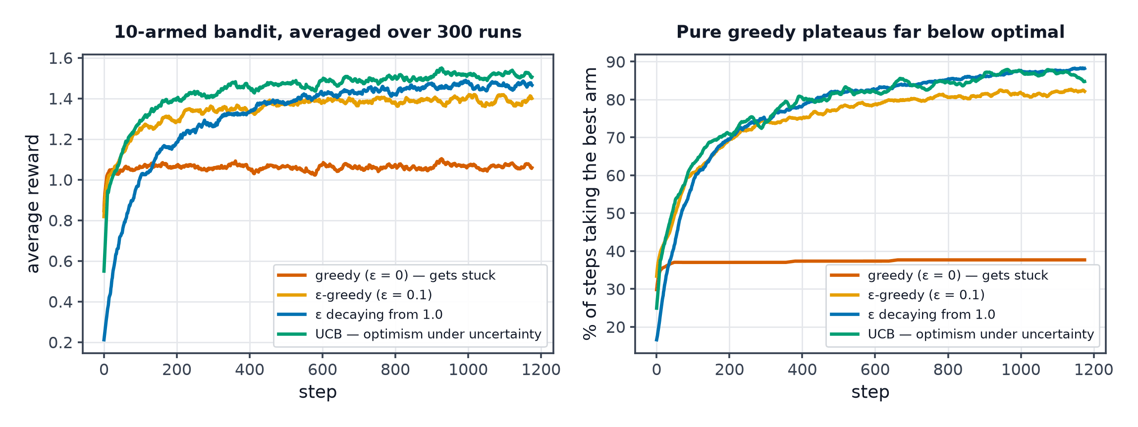
The exploration/exploitation dilemma stated

Every action choice is implicitly a trade-off: exploit the action currently believed best, guaranteeing (as far as current beliefs go) good short-term return, or explore an uncertain alternative, risking worse short-term return in exchange for potentially discovering something even better. No fixed strategy is unconditionally correct — the right balance depends on how much time remains to exploit any discovery.

Multi-armed bandits as the minimal setting

A multi-armed bandit strips away everything except the exploration problem itself: $k$ actions ("arms"), no state transitions, and a stationary (unknown) reward distribution per arm — pure "which arm should I pull next," with no Markov Decision Processes-style state to complicate things. Every exploration method in this section is introduced here first, in this simplest possible setting.

Regret as the measure

$$\text{Regret}(T) = \sum_{t=1}^{T} \left( \mu^* - \mu_{a_t} \right)$$

Regret measures the total reward lost, over $T$ pulls, relative to always having pulled the single best arm $\mu^*$ from the start. A good exploration strategy should have regret that grows sub-linearly in $T$ — meaning the average regret per step shrinks toward zero as more is learned, rather than accumulating a constant per-step penalty forever.

ε-greedy and its decay schedules

As in Q-Learning and SARSA: with probability $\varepsilon$, act randomly; otherwise exploit. A fixed $\varepsilon$ incurs linear regret (a constant fraction of steps stays random forever); decaying $\varepsilon$ (shrinking it over time, e.g. $\varepsilon_t = 1/t$) can achieve sub-linear regret, since exploration naturally tapers off as confidence in the best arm grows.

Optimistic initialisation

Initialise every action's estimated value above what's realistically achievable. Every arm looks attractive at first purely because its estimate hasn't been "disappointed" by real experience yet — this alone drives the agent to try every arm at least once early on, achieving a simple form of directed exploration with no explicit randomness needed.

Upper confidence bounds, and the intuition behind the bonus term

$$a_t = \arg\max_a \left[ \hat\mu_a + c \sqrt{\frac{\ln t}{N_a}} \right]$$

UCB adds an explicit uncertainty bonus to each arm's estimated value $\hat\mu_a$ — larger for arms pulled fewer times ($N_a$ small), shrinking as an arm is pulled more (more confidence in its estimate). The principle: optimism in the face of uncertainty — act as if uncertain arms might be as good as their most optimistic plausible value, which naturally directs exploration toward arms that are both promising and under-explored.

Thompson sampling

Maintain a full posterior distribution over each arm's true reward (a Bayesian belief, updated after every pull), and at each step, sample one value from each arm's posterior and act greedily with respect to those samples. An arm with high uncertainty (a wide posterior) occasionally samples a high value purely by chance, driving exploration — and this exploration naturally and automatically tapers off as posteriors narrow with more data, with no separately-tuned schedule required.

Boltzmann/softmax exploration

Rather than binary random-or-greedy (ε-greedy), select actions probabilistically, weighted by their estimated value via a softmax with temperature $\tau$: higher-valued actions are more likely but not certain, and the temperature directly controls how sharply the distribution concentrates on the current best estimate.

Entropy bonuses in policy gradient methods

Policy Gradient Methods's entropy regularisation is exploration expressed differently: rather than randomness bolted onto a deterministic decision rule, the policy's own natural stochasticity provides exploration directly, with the entropy bonus in the objective preventing it from collapsing to deterministic too early.

The hard-exploration problem

Sparse rewards: almost every state gives zero reward, with a single distant informative signal — none of the methods above provide any directed guidance toward that signal; they explore roughly uniformly (or by uncertainty) with no sense of where the reward might actually be. Deceptive rewards: a locally-appealing but ultimately suboptimal reward signal actively misleads naive exploration away from a better distant solution — a genuinely harder problem than sparsity alone.

Count-based and pseudo-count bonuses

Add an exploration bonus inversely proportional to how many times a state has been visited — directly generalising UCB's bonus term from bandit arms to full states, giving the agent an explicit incentive to visit novel states specifically. For large or continuous state spaces where exact counts are meaningless (no state repeats exactly), pseudo-counts estimate an effective visit count using a density model's change in predicted probability after seeing a state.

Curiosity and prediction-error intrinsic rewards, plus the noisy-TV failure

Curiosity-driven exploration: train an auxiliary model to predict the next state from the current state and action, and use the prediction error as an intrinsic reward — states the agent can't yet predict well are, by this measure, novel and worth visiting. The well-documented noisy-TV problem: if part of the environment is genuinely unpredictable (pure noise, not learnable structure), a curiosity-driven agent can become permanently fixated on it, since prediction error there never decreases no matter how much it's visited — a directed exploration signal that is not, in fact, always leading toward useful learning.

When reward shaping is the honest answer instead

If the designer actually knows something about where useful behaviour lies, explicit reward shaping (RL Problem Setup) — hand-designing denser intermediate rewards — can be a more honest and effective solution than any general-purpose exploration bonus, provided it's done carefully enough to avoid the reward-hacking failure modes already covered. Exploration bonuses are the right tool when no such prior knowledge is available; shaping is the right tool when it is.

A selection table

Method	Best suited for
ε-greedy (decayed)	simple discrete-action baseline
UCB	small discrete action sets, strong theoretical guarantees wanted
Thompson sampling	when a good prior/posterior model is available
Entropy bonus	policy-gradient methods, continuous or large action spaces
Count/curiosity bonuses	sparse-reward, large state spaces

Symbol	Meaning
$\mu_a, \hat\mu_a$	true and estimated mean reward of arm $a$
$N_a$	number of times arm $a$ has been pulled
$\text{Regret}(T)$	cumulative regret after $T$ steps

Code: ε-greedy, UCB, and Thompson sampling compared on a 10-armed bandit

exploration_strategies_demo.py

import numpy as np
import matplotlib.pyplot as plt

rng = np.random.default_rng(0)
n_arms, n_steps = 10, 2000
true_means = rng.normal(0, 1, n_arms)
best_arm_mean = true_means.max()

def epsilon_greedy_bandit(epsilon=0.1):
    Q, N = np.zeros(n_arms), np.zeros(n_arms)
    regrets = []
    for t in range(1, n_steps + 1):
        arm = rng.integers(n_arms) if rng.random() < epsilon else np.argmax(Q)
        reward = rng.normal(true_means[arm], 1)
        N[arm] += 1
        Q[arm] += (reward - Q[arm]) / N[arm]
        regrets.append(best_arm_mean - true_means[arm])
    return np.cumsum(regrets)

def ucb_bandit(c=2.0):
    Q, N = np.zeros(n_arms), np.zeros(n_arms)
    regrets = []
    for t in range(1, n_steps + 1):
        if t <= n_arms:
            arm = t - 1  # pull each arm once first
        else:
            bonus = c * np.sqrt(np.log(t) / N)
            arm = np.argmax(Q + bonus)
        reward = rng.normal(true_means[arm], 1)
        N[arm] += 1
        Q[arm] += (reward - Q[arm]) / N[arm]
        regrets.append(best_arm_mean - true_means[arm])
    return np.cumsum(regrets)

def thompson_sampling_bandit():
    # Gaussian bandit with a Gaussian posterior over each arm's mean (known unit variance)
    posterior_mean, posterior_precision = np.zeros(n_arms), np.ones(n_arms)
    regrets = []
    for t in range(n_steps):
        samples = rng.normal(posterior_mean, 1 / np.sqrt(posterior_precision))
        arm = np.argmax(samples)
        reward = rng.normal(true_means[arm], 1)
        posterior_precision[arm] += 1
        posterior_mean[arm] += (reward - posterior_mean[arm]) / posterior_precision[arm]
        regrets.append(best_arm_mean - true_means[arm])
    return np.cumsum(regrets)

plt.plot(epsilon_greedy_bandit(), label="epsilon-greedy")
plt.plot(ucb_bandit(), label="UCB")
plt.plot(thompson_sampling_bandit(), label="Thompson sampling")
plt.xlabel("step"); plt.ylabel("cumulative regret")
plt.legend(); plt.title("exploration strategies on a 10-armed bandit")
plt.savefig("bandit_regret_comparison.png")

See also

• Q-Learning and SARSA — where ε-greedy exploration was first introduced in the MDP setting.
• The Reinforcement Learning Problem — the exploration/exploitation dilemma, first introduced.