Markov Decision Processes

The Reinforcement Learning Problem described the agent-environment loop informally. The Markov Decision Process (MDP) is the formalism that makes that loop mathematically precise — and precise enough that every algorithm in this section can be stated and analysed against it.

Key idea

If the current state contains everything relevant about the past, the optimal action depends only on where you are - not on how you got there.

A 4×4 gridworld solved by value iteration. The values and arrows are computed, not drawn — note the cell below the trap points *down and away* from the +1 goal, because reaching it via the trap is worse than the longer route.

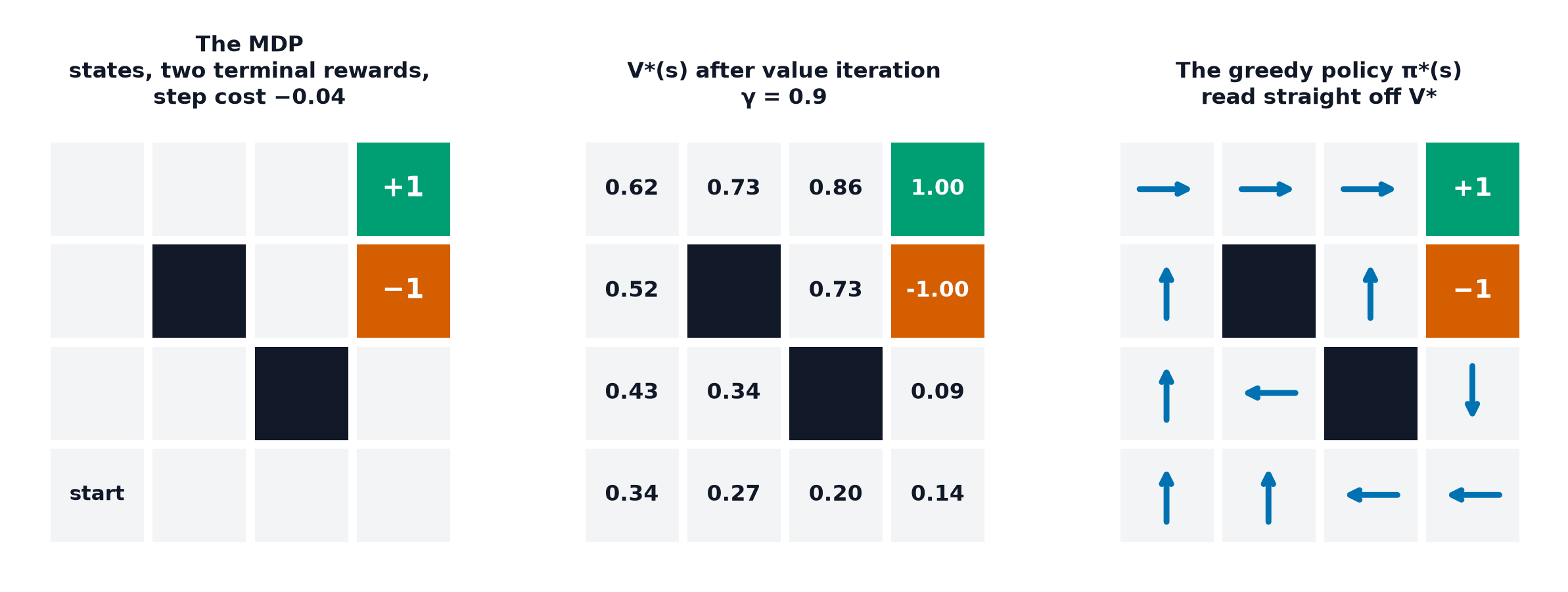
The MDP tuple (S, A, P, R, γ)

An MDP is defined by five components: the state space $\mathcal{S}$, the action space $\mathcal{A}$, the transition function $P(s' \mid s, a)$, the reward function $R(s, a, s')$, and the discount factor $\gamma$. Together, this tuple fully specifies the environment's dynamics — everything an agent could possibly need to know about how the world responds to its actions.

The Markov property, and what it rules out

A state $s_t$ is Markov if $P(s_{t+1} \mid s_t, a_t) = P(s_{t+1} \mid s_1, a_1, \dots, s_t, a_t)$ — the next state depends only on the current state and action, not on the full history that led there. This rules out any environment where the sequence of past states matters beyond what's captured in the current state — a genuinely restrictive assumption, and one real problems frequently violate (addressed below).

Transition and reward functions

$P(s' \mid s, a)$ gives the probability of landing in state $s'$ after taking action $a$ in state $s$ — the environment's dynamics, and generally unknown to the agent. $R(s, a, s')$ gives the (expected) reward received for that transition. Together they define everything about "how the world works," separate entirely from the policy the agent uses to choose actions.

Policies: deterministic and stochastic

A policy $\pi$ maps states to actions. Deterministic: $\pi(s) = a$, a fixed choice per state. Stochastic: $\pi(a \mid s)$, a probability distribution over actions per state — necessary for methods that need to explore (visiting different actions in the same state across episodes) or that arise naturally from policy-gradient optimisation (Policy Gradient Methods).

Trajectories and their probability

A trajectory $\tau = (s_0, a_0, r_1, s_1, a_1, r_2, \dots)$ is one full run through the MDP under a given policy. Because of the Markov property, its probability factorises cleanly:

$$P(\tau \mid \pi) = P(s_0) \prod_{t=0}^{T-1} \pi(a_t \mid s_t) \, P(s_{t+1} \mid s_t, a_t)$$

The objective: expected return

γ sets how far ahead the agent effectively plans — roughly 1/(1−γ) steps. At γ = 0.9 a reward fifty steps away is worth half a percent of an immediate one, so the agent is functionally blind to it.

$$J(\pi) = \mathbb{E}_{\tau \sim \pi} \left[ G_0 \right] = \mathbb{E}_{\tau \sim \pi} \left[ \sum_{t=0}^{\infty} \gamma^t r_{t+1} \right]$$

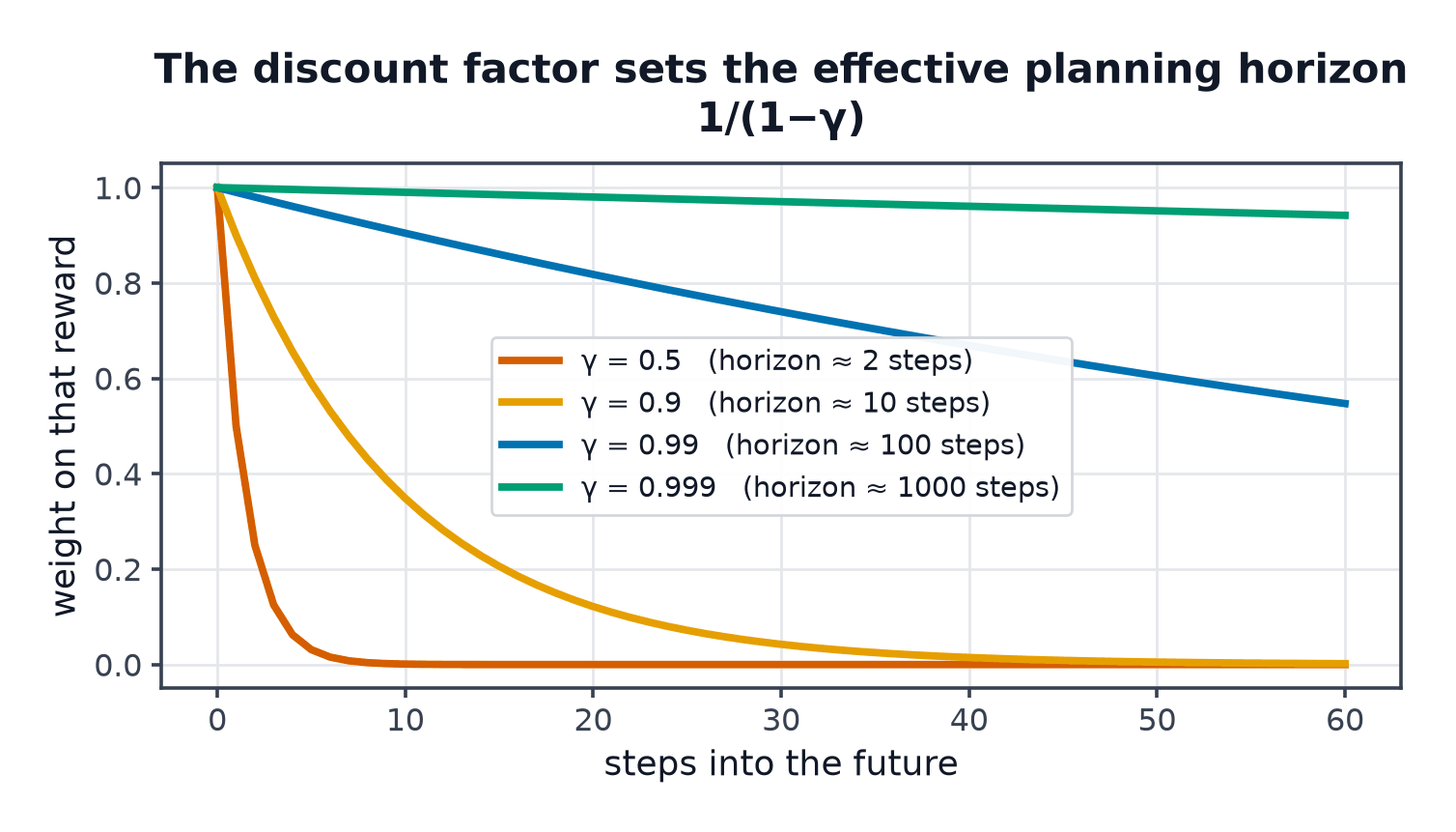
Every RL algorithm, regardless of family, is ultimately trying to find a policy $\pi$ that maximises this single quantity — the expected discounted return over trajectories the policy would generate.

Partial observability and POMDPs, briefly

Real problems often violate the Markov property directly: the agent's observation may not contain everything relevant (a robot's camera doesn't see behind it; a poker player doesn't see opponents' cards). A POMDP (Partially Observable MDP) formalises this by separating the true (hidden) state from the agent's observation. A common practical workaround, rather than solving the full POMDP machinery: frame-stacking — feed the agent a short history of recent observations instead of just the current one, which often restores enough Markov-like structure for standard MDP methods to work reasonably well.

Finite vs. continuous state and action spaces

Finite: both $\mathcal{S}$ and $\mathcal{A}$ are discrete and enumerable (this section's grid world). Continuous: either or both are real-valued (a robot's joint angles, a steering command). Tabular methods (Dynamic Programming, Q-Learning and SARSA) require finite spaces; continuous spaces require function approximation, which is exactly why Deep Q-Networks onward exist.

What "solving" an MDP means

Solving an MDP means finding an optimal policy $\pi^*$ — one that achieves the maximum possible expected return from every state simultaneously. This is a stronger requirement than merely finding a good policy for one particular starting state; a genuinely optimal policy is optimal everywhere at once.

The existence of an optimal deterministic policy

For any finite MDP, there exists at least one optimal policy that is deterministic — a real, useful theoretical guarantee: even though stochastic policies are sometimes convenient computationally (for exploration, for gradient-based optimisation), you never need randomness to achieve optimal expected return in a fully-observed finite MDP.

How real problems are forced into this frame, and what gets lost

Applying MDP theory to a real problem requires choosing a state representation, a reward function, and often a discretisation of continuous quantities — each of these choices can silently discard information the true Markov property would need, or bake in a reward function that doesn't perfectly capture the intended goal (RL Problem Setup's reward-hacking discussion). The mathematical elegance of the MDP formalism is genuine, but it depends entirely on the modelling choices made before any algorithm runs.

Symbol	Meaning
$\mathcal{S}, \mathcal{A}$	state space and action space
$P(s' \mid s, a)$	transition function
$R(s, a, s')$	reward function
$\pi(a \mid s)$	policy

Code: the grid world as explicit transition and reward matrices

mdp_demo.py

import numpy as np
from grid_world_env import GridWorld

env = GridWorld(size=4)
n_states = env.size * env.size
n_actions = 4

def state_to_index(pos):
    return pos[0] * env.size + pos[1]

# --- Build P[s, a, s'] and R[s, a] explicitly from the environment's dynamics ---
P = np.zeros((n_states, n_actions, n_states))
R = np.zeros((n_states, n_actions))
for r in range(env.size):
    for c in range(env.size):
        s = state_to_index((r, c))
        for a in range(n_actions):
            env.pos = (r, c)
            next_pos, reward, done = env.step(a)
            s_next = state_to_index(next_pos)
            P[s, a, s_next] = 1.0  # deterministic transitions in this grid world
            R[s, a] = reward

# --- A fixed policy: always move toward the goal (down, then right) ---
policy = np.zeros((n_states, n_actions))
for r in range(env.size):
    for c in range(env.size):
        s = state_to_index((r, c))
        action = 1 if r < env.size - 1 else 3  # down until aligned, then right
        policy[s, action] = 1.0

# --- Probability of one specific 3-step trajectory under this policy, computed by hand ---
trajectory = [((0, 0), 1), ((1, 0), 1), ((2, 0), 1)]  # (state, action) pairs
prob = 1.0
for pos, action in trajectory:
    s = state_to_index(pos)
    prob *= policy[s, action]
print(f"probability of this specific trajectory under the policy: {prob:.3f}")
print(f"transition matrix shape: {P.shape}, reward matrix shape: {R.shape}")

See also

• Value Functions and Bellman Equations — the recursive machinery built directly on this tuple.
• The Reinforcement Learning Problem — the informal version of the loop this page formalises.