PPO and Trust Regions

Every algorithm so far has taken a plain gradient step on the policy — and a plain gradient step, if it's too large, can destroy the policy in a way a large supervised-learning update never does. Proximal Policy Optimization is the algorithm most production RL systems actually run, and its entire design is built around preventing exactly that failure.

Key idea

A policy update that is too large destroys the policy irrecoverably, so constrain how far each update is allowed to move.

The PPO clipped objective plotted against the probability ratio for positive and negative advantage — PPO's clipping flattens the objective once the policy ratio leaves [1−ε, 1+ε], so there is no gradient rewarding a further move. That is what keeps the update inside a trust region without TRPO's second-order machinery.

Why a large policy update is catastrophic in a way a large supervised update is not

In supervised learning, a bad gradient step produces a worse model on a fixed dataset — recoverable, since the next step sees the same data again. In RL, the data itself comes from the current policy: a large, destructive update produces a bad policy, which then generates bad, uninformative trajectories, which then makes it hard to even get a useful gradient to recover — the data distribution moves with the policy, and a bad enough move can be effectively irreversible.

The trust region idea

Rather than taking an unconstrained gradient step, constrain each update to stay within a trust region — a neighbourhood around the current policy where the approximation used to compute the update is still believed to be accurate — trading off some update size for guaranteed (or empirically reliable) improvement, or at least no catastrophic regression.

TRPO and the KL constraint, stated

TRPO (Trust Region Policy Optimization) formalises this directly: maximise the policy improvement objective subject to an explicit constraint that the KL divergence between the old and new policy stays below a threshold $\delta$ :

\max_\theta \; \mathbb{E}\left[ \frac{\pi_\theta(a\mid s)}{\pi_{\theta_{\text{old}}}(a\mid s)} \hat A \right] \quad \text{subject to} \quad \mathbb{E}\left[ D_{KL}(\pi_{\theta_{\text{old}}} \| \pi_\theta) \right] \leq \delta

Solving this constrained optimisation exactly requires second-order methods (conjugate gradient, a Fisher-information matrix computation) — theoretically principled, but computationally expensive and fiddly to implement correctly.

The surrogate objective and the importance-sampling ratio

r_t(\theta) = \frac{\pi_\theta(a_t \mid s_t)}{\pi_{\theta_{\text{old}}}(a_t \mid s_t)}

The importance-sampling ratio $r_t(\theta)$ corrects for the fact that trajectories were collected under the old policy but are being used to estimate the new policy's objective — a standard technique for reusing off-distribution samples, here applied to reuse the same batch across multiple gradient steps.

PPO's clipped objective as a first-order approximation of the same idea

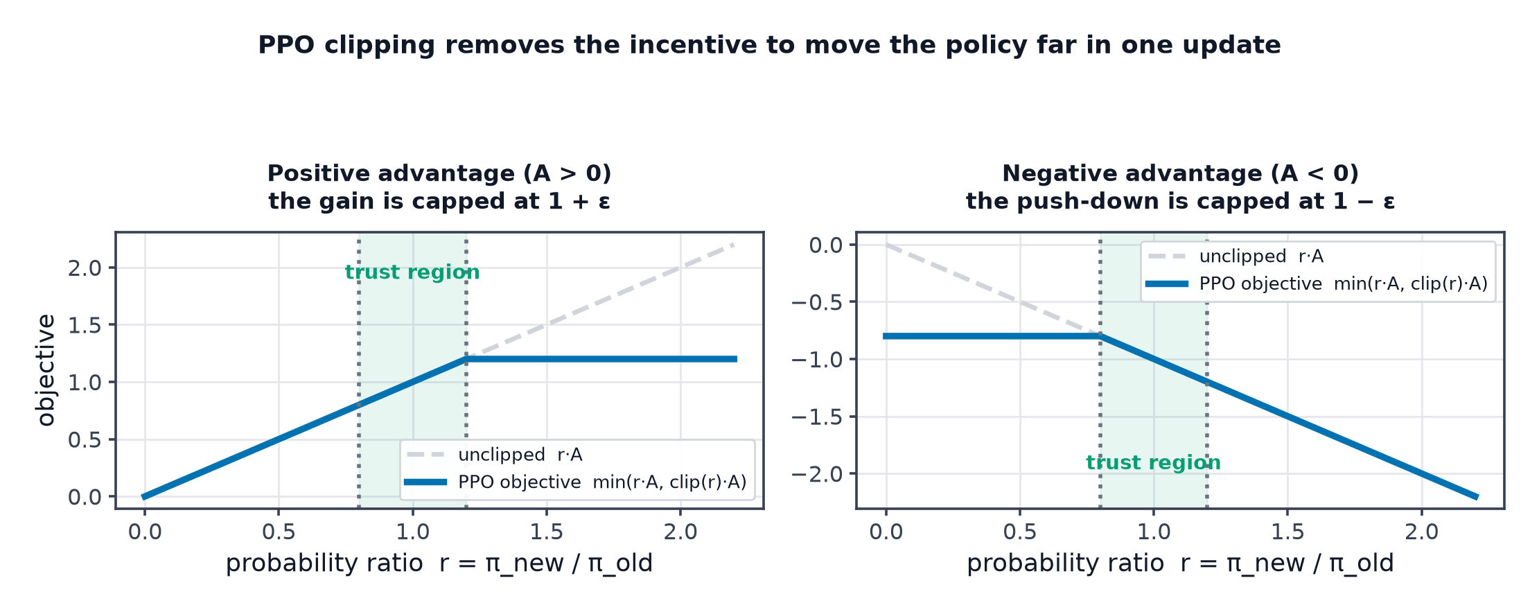
L^{\text{CLIP}}(\theta) = \mathbb{E}\left[ \min\left( r_t(\theta) \hat A_t,\ \text{clip}(r_t(\theta), 1-\epsilon, 1+\epsilon) \hat A_t \right) \right]

PPO achieves a similar effect to TRPO's hard KL constraint — discouraging updates that move the policy too far — using nothing more than a clipped ratio and first-order gradient descent, with no second-order machinery required. Simpler to implement correctly, and empirically competitive with TRPO's performance.

Why clipping works, and what it actually prevents

The $\min$ of the unclipped and clipped terms means: when the advantage is positive (a good action, worth reinforcing), the objective stops rewarding the update once the ratio exceeds $1+\epsilon$ — no incentive to push the policy arbitrarily far in that direction. When the advantage is negative, the symmetric floor at $1-\epsilon$ applies. The clip specifically removes the incentive for the optimiser to move too far in either direction — it does not literally cap how far a single gradient step could move parameters, but it removes the objective's reward for doing so.

Multiple epochs over the same batch, and the sample-efficiency gain

Because the clipped objective explicitly discourages the ratio from drifting too far from 1, PPO can safely take several gradient epochs over the same collected batch of trajectories before discarding it and collecting new data — extracting more learning signal per environment interaction than a single-epoch update would, a meaningful sample-efficiency improvement for an otherwise-on-policy method.

The PPO hyperparameters that matter

Clip range $\epsilon$ : typically 0.1–0.3, controlling how far the ratio is allowed to drift. Epochs: how many passes over each batch before discarding it. Batch size: how much experience is collected per update. GAE λ: the bias/variance dial from Actor-Critic Methods. Entropy coefficient: how strongly exploration is encouraged via the entropy bonus.

The implementation details that dominate reported performance

Empirically, several "minor" implementation choices matter as much as the core algorithm: observation normalisation (running mean/std of observations, keeping inputs well-scaled), advantage normalisation (per-batch standardisation of advantages, stabilising the gradient scale), and value function clipping (an analogous clip applied to the critic's updates). Papers reproducing PPO results that omit these often see substantially worse performance — the algorithm's paper-level description is not the whole story.

PPO in RLHF

PPO's stability and sample-reuse make it the standard choice for the RL stage of RLHF (RLHF and Preference Optimization) — treating the language model itself as the policy, with a learned reward model providing the reward signal, and a KL penalty against a reference model serving a role closely related to this page's trust-region idea (preventing the fine-tuned model from drifting too far from its starting point).

A diagnosis table for a PPO run that is not improving

Symptom	Likely cause
Return flat from the start	learning rate too low, or reward signal too sparse
Return rises then collapses	clip range too wide, or too many epochs per batch
High variance across seeds	batch size too small, advantage not normalised
KL divergence exploding despite clipping	clip range too wide relative to policy's sensitivity

Symbol	Meaning
$r_t(\theta)$	the importance-sampling probability ratio
$\epsilon$	the PPO clip range
$\hat A_t$	the advantage estimate (typically via GAE)

Code: a complete PPO implementation on CartPole, the clip visualised, a clip-range sweep

ppo_demo.py
import torch
import torch.nn as nn
import numpy as np
import matplotlib.pyplot as plt
from deep_q_network_demo import TinyCartPole
from policy_gradient_demo import PolicyNetwork, ValueNetwork, run_episode
from actor_critic_demo import compute_gae

def train_ppo(clip_range=0.2, n_updates=100, epochs_per_update=4):
    env = TinyCartPole()
    actor = PolicyNetwork()
    critic = ValueNetwork()
    actor_opt = torch.optim.Adam(actor.parameters(), lr=0.005)
    critic_opt = torch.optim.Adam(critic.parameters(), lr=0.005)
    returns_log = []

    for update in range(n_updates):
        states, actions, rewards = run_episode(env, actor)
        states_t = torch.tensor(np.array(states), dtype=torch.float32)
        actions_t = torch.tensor(actions)

        with torch.no_grad():
            old_probs = actor(states_t).gather(1, actions_t.unsqueeze(1)).squeeze(1)
            values = critic(states_t).tolist()
        advantages = torch.tensor(compute_gae(rewards, values, 0.0), dtype=torch.float32)
        advantages = (advantages - advantages.mean()) / (advantages.std() + 1e-8)  # advantage normalisation
        returns_target = advantages + torch.tensor(values, dtype=torch.float32)

        for epoch in range(epochs_per_update):  # multiple epochs over the same batch
            new_probs = actor(states_t).gather(1, actions_t.unsqueeze(1)).squeeze(1)
            ratio = new_probs / (old_probs + 1e-8)
            unclipped = ratio * advantages
            clipped = torch.clamp(ratio, 1 - clip_range, 1 + clip_range) * advantages
            actor_loss = -torch.min(unclipped, clipped).mean()
            actor_opt.zero_grad(); actor_loss.backward(); actor_opt.step()

            value_loss = nn.functional.mse_loss(critic(states_t), returns_target)
            critic_opt.zero_grad(); value_loss.backward(); critic_opt.step()

        returns_log.append(sum(rewards))
    return returns_log

# --- Clip-range sweep ---
fig, ax = plt.subplots(figsize=(8, 4))
for clip_range in [0.1, 0.2, 0.4]:
    returns = train_ppo(clip_range=clip_range)
    window = 10
    smoothed = np.convolve(returns, np.ones(window) / window, mode="valid")
    ax.plot(smoothed, label=f"clip={clip_range}")
ax.set_xlabel("update"); ax.set_ylabel("smoothed return")
ax.legend(); ax.set_title("PPO clip-range sweep on CartPole")
plt.savefig("ppo_clip_range_sweep.png")

# --- Visualise where the clipped objective zeroes gradients relative to the ratio ---
ratios = np.linspace(0.5, 1.5, 200)
advantage_pos, advantage_neg = 1.0, -1.0
clipped_pos = np.minimum(ratios * advantage_pos, np.clip(ratios, 0.8, 1.2) * advantage_pos)
clipped_neg = np.minimum(ratios * advantage_neg, np.clip(ratios, 0.8, 1.2) * advantage_neg)
fig2, ax2 = plt.subplots()
ax2.plot(ratios, clipped_pos, label="advantage > 0")
ax2.plot(ratios, clipped_neg, label="advantage < 0")
ax2.axvline(0.8, linestyle="--", color="gray"); ax2.axvline(1.2, linestyle="--", color="gray")
ax2.set_xlabel("probability ratio r(theta)"); ax2.set_ylabel("clipped objective")
ax2.legend(); ax2.set_title("where clipping flattens the objective (zero gradient)")
plt.savefig("ppo_clipped_objective.png")

Why a large policy update is catastrophic in a way a large supervised update is not​

The trust region idea​

TRPO and the KL constraint, stated​

The surrogate objective and the importance-sampling ratio​

PPO's clipped objective as a first-order approximation of the same idea​

Why clipping works, and what it actually prevents​

Multiple epochs over the same batch, and the sample-efficiency gain​

The PPO hyperparameters that matter​

The implementation details that dominate reported performance​

PPO in RLHF​

A diagnosis table for a PPO run that is not improving​

Code: a complete PPO implementation on CartPole, the clip visualised, a clip-range sweep​

See also​