Q-Learning and SARSA

Monte Carlo and TD Learning only evaluated a fixed policy. This page turns TD prediction into control — algorithms that learn to act well, with no model of the environment — and the two most fundamental such algorithms differ by exactly one term in their update rule.

Key idea

SARSA learns the value of the policy it is following; Q-learning learns the value of the best policy regardless of what it is following - one word of difference in the update.

From prediction to control

Prediction estimates $V^\pi$ or $Q^\pi$ for a fixed policy. Control interleaves that estimation with policy improvement — exactly Value Functions and Bellman Equations's generalised policy iteration, but now using TD updates from real experience instead of full DP sweeps.

ε-greedy action selection

To learn $Q^\pi$ for a policy that's simultaneously supposed to be improving toward optimal, the agent needs to keep exploring even as it gets better. ε-greedy: with probability $1-\varepsilon$ take the currently-best action ($\arg\max_a Q(s,a)$); with probability $\varepsilon$ take a uniformly random action instead — a simple, effective way to guarantee continued exploration without abandoning exploitation entirely.

SARSA: the on-policy update

$$Q(s_t, a_t) \leftarrow Q(s_t, a_t) + \alpha \left[ r_{t+1} + \gamma Q(s_{t+1}, a_{t+1}) - Q(s_t, a_t) \right]$$

Named for the quintuple it needs: $(s_t, a_t, r_{t+1}, s_{t+1}, a_{t+1})$. Critically, $a_{t+1}$ is the action the current, exploring policy actually selects next — SARSA evaluates and improves the same policy it's using to act, making it on-policy.

Q-learning: the off-policy update

$$Q(s_t, a_t) \leftarrow Q(s_t, a_t) + \alpha \left[ r_{t+1} + \gamma \max_{a'} Q(s_{t+1}, a') - Q(s_t, a_t) \right]$$

The only difference: instead of the action the exploring policy actually takes next, Q-learning bootstraps using $\max_{a'} Q(s_{t+1}, a')$ — the value of the best possible next action, regardless of what the exploring behaviour policy would actually do. Q-learning learns about the optimal (greedy) policy while following an entirely different (exploratory) one — off-policy.

The single-term difference between the two, and everything that follows from it

	SARSA	Q-learning
Bootstrap target	$Q(s_{t+1}, a_{t+1})$, the action actually taken	$\max_{a'} Q(s_{t+1}, a')$, the best possible action
On/off-policy	on-policy	off-policy
Learns the value of	the policy being followed (including exploration)	the optimal greedy policy

That single substituted term changes what each algorithm is actually optimising for — SARSA's learned values account for the exploration it will keep doing; Q-learning's do not.

The cliff-walking example

The classic separation between the two. Q-learning learns the optimal path and hugs the cliff; SARSA learns the value of the ε-greedy policy it actually follows, so it accounts for the chance of a random step into the cliff and detours. Under exploration SARSA therefore earns more — −25 against −53 in this run.

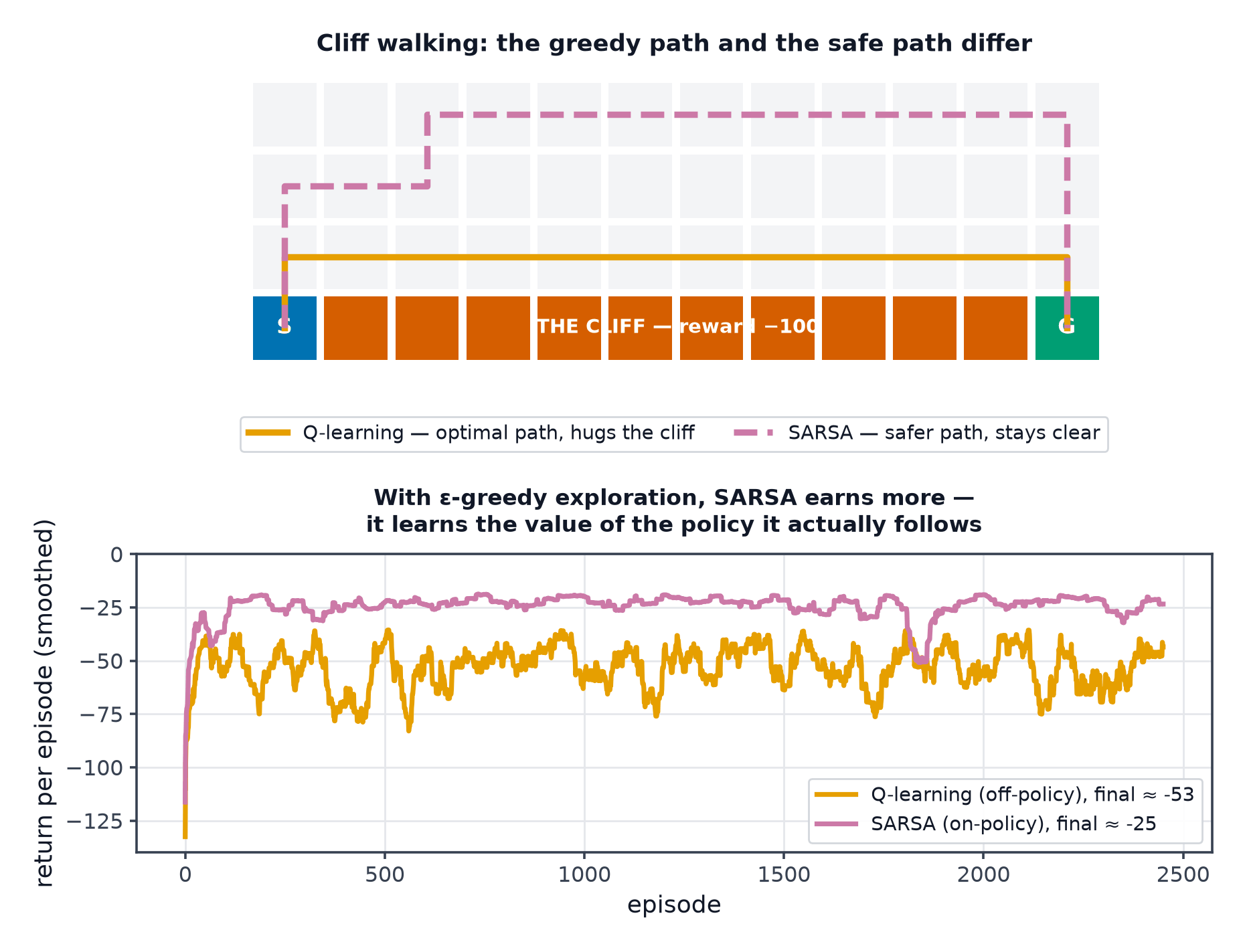
On a grid with a cliff running along one edge (stepping into it ends the episode with a large penalty), SARSA — because it accounts for its own ε-greedy exploration in its value estimates — learns a safe path that stays away from the cliff edge, since an exploratory random step near the edge would be catastrophic. Q-learning, evaluating the purely greedy optimal policy regardless of the exploration actually used, learns the risky, optimal path directly along the cliff edge — and then, still exploring with ε-greedy during training, occasionally falls in. This is the canonical illustration of the on/off-policy distinction actually mattering for real behaviour, not just as a theoretical label.

Expected SARSA

A variant that replaces SARSA's sampled $Q(s_{t+1}, a_{t+1})$ with its full expectation under the current policy: $\sum_{a'} \pi(a' \mid s_{t+1}) Q(s_{t+1}, a')$ — reduces variance relative to plain SARSA (no dependence on which specific action happened to be sampled) while remaining on-policy, at the cost of computing a sum over all actions each update.

Convergence conditions, and why they rarely hold in practice

Both algorithms are guaranteed to converge to $Q^*$ under tabular representation, given every state-action pair visited infinitely often and a learning rate satisfying the Robbins-Monro conditions ($\sum \alpha_t = \infty$, $\sum \alpha_t^2 < \infty$). In practice, learning rates are fixed or decayed heuristically, and state spaces are far too large to visit every pair infinitely often — the theoretical guarantees are a useful sanity check, not a practical promise.

Maximisation bias and double Q-learning

Q-learning's $\max_{a'} Q(s_{t+1}, a')$ tends to systematically overestimate true action values — because $Q$ itself is a noisy estimate, taking the max over noisy estimates is biased upward (the same statistical effect as the max of several noisy measurements exceeding the true maximum in expectation). Double Q-learning fixes this by maintaining two independent $Q$-estimates, using one to select the best action and the other to evaluate it — decoupling selection from evaluation removes the systematic bias.

The tabular ceiling: what happens when the state space is large

Every algorithm on this page stores $Q$ as an explicit table, indexed by state and action — completely infeasible once states are continuous or combinatorially large (an image, a robot's joint configuration). This is the tabular ceiling every method here runs into identically.

This is where function approximation becomes necessary

Replacing the table with a parameterised function (a neural network) that generalises across similar states — rather than storing a separate value for every state independently — is exactly what Deep Q-Networks does next, and it introduces genuinely new instability problems that tabular Q-learning never has to deal with.

Symbol	Meaning
$\varepsilon$	the exploration probability in ε-greedy
$Q(s,a)$	the tabular action-value estimate being learned

Code: SARSA and Q-learning on cliff-walking, safe vs. optimal paths

q_learning_sarsa_demo.py

import numpy as np
import matplotlib.pyplot as plt

class CliffWalk:
    """4x12 grid: start bottom-left, goal bottom-right, cliff along the bottom edge between them."""
    def __init__(self):
        self.rows, self.cols = 4, 12
        self.start, self.goal = (3, 0), (3, 11)
        self.cliff = {(3, c) for c in range(1, 11)}
        self.actions = {0: (-1, 0), 1: (1, 0), 2: (0, -1), 3: (0, 1)}

    def reset(self):
        self.pos = self.start
        return self.pos

    def step(self, action):
        dr, dc = self.actions[action]
        r, c = self.pos
        new_pos = (min(max(r + dr, 0), self.rows - 1), min(max(c + dc, 0), self.cols - 1))
        if new_pos in self.cliff:
            return self.start, -100.0, True
        self.pos = new_pos
        done = new_pos == self.goal
        return new_pos, -1.0, done

def s_idx(pos, cols=12):
    return pos[0] * cols + pos[1]

def epsilon_greedy(Q, s, epsilon, rng):
    return rng.integers(4) if rng.random() < epsilon else np.argmax(Q[s])

def run_sarsa(env, n_episodes=500, alpha=0.5, gamma=1.0, epsilon=0.1):
    Q = np.zeros((env.rows * env.cols, 4))
    rng = np.random.default_rng(0)
    returns = []
    for ep in range(n_episodes):
        state = env.reset()
        s = s_idx(state)
        action = epsilon_greedy(Q, s, epsilon, rng)
        total_return = 0.0
        for _ in range(200):
            next_state, reward, done = env.step(action)
            s_next = s_idx(next_state)
            next_action = epsilon_greedy(Q, s_next, epsilon, rng)
            Q[s, action] += alpha * (reward + gamma * Q[s_next, next_action] - Q[s, action])
            s, action = s_next, next_action
            total_return += reward
            if done:
                break
        returns.append(total_return)
    return Q, returns

def run_q_learning(env, n_episodes=500, alpha=0.5, gamma=1.0, epsilon=0.1):
    Q = np.zeros((env.rows * env.cols, 4))
    rng = np.random.default_rng(0)
    returns = []
    for ep in range(n_episodes):
        state = env.reset()
        s = s_idx(state)
        total_return = 0.0
        for _ in range(200):
            action = epsilon_greedy(Q, s, epsilon, rng)
            next_state, reward, done = env.step(action)
            s_next = s_idx(next_state)
            Q[s, action] += alpha * (reward + gamma * Q[s_next].max() - Q[s, action])
            s = s_next
            total_return += reward
            if done:
                break
        returns.append(total_return)
    return Q, returns

env = CliffWalk()
Q_sarsa, returns_sarsa = run_sarsa(env)
Q_qlearning, returns_qlearning = run_q_learning(env)

fig, ax = plt.subplots(figsize=(8, 4))
window = 20
ax.plot(np.convolve(returns_sarsa, np.ones(window) / window, mode="valid"), label="SARSA (safe path)")
ax.plot(np.convolve(returns_qlearning, np.ones(window) / window, mode="valid"), label="Q-learning (risky optimal path)")
ax.set_xlabel("episode"); ax.set_ylabel("smoothed return")
ax.legend(); ax.set_title("SARSA's caution vs Q-learning's risk, both under epsilon-greedy exploration")
plt.savefig("cliff_walking_sarsa_vs_qlearning.png")

See also

• Deep Q-Networks — replacing the Q-table with a neural network to escape the tabular ceiling.
• Exploration Strategies — alternatives to ε-greedy for the exploration this page relies on.