Value Functions and Bellman Equations

"How good is this state?" sounds unanswerable without simulating every possible future — except it isn't, because of a recursive identity that turns an infinite lookahead into a one-step relationship. That identity, the Bellman equation, is the single mathematical tool every algorithm in this section exploits in some form.

Key idea

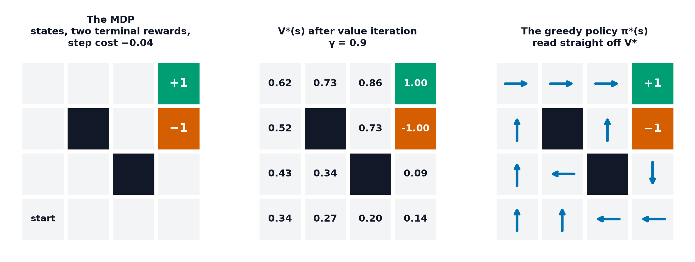
The value of a state equals the immediate reward plus the discounted value of what comes next; every algorithm in this section exploits that recursion.

V*(s) is the expected return from each state under optimal play. Once you have it the policy is free: at every state, take the action leading to the highest-valued neighbour — which is what the arrows in the third panel are.

The state-value function V^π

$$V^\pi(s) = \mathbb{E}_\pi \left[ G_t \mid s_t = s \right]$$

The expected return, starting from state $s$, if the agent follows policy $\pi$ thereafter — a single number per state, summarising "how good is it to be here, given how I'll act from now on."

The action-value function Q^π

$$Q^\pi(s, a) = \mathbb{E}_\pi \left[ G_t \mid s_t = s, a_t = a \right]$$

The expected return from taking a specific action $a$ in state $s$, then following $\pi$ thereafter — one level more specific than $V^\pi$, and, as later pages show, the more directly useful quantity for actually choosing actions.

The relationship between them

$$V^\pi(s) = \sum_a \pi(a \mid s) \, Q^\pi(s, a)$$

$V^\pi$ is exactly the expectation of $Q^\pi$ over the policy's action distribution — knowing $Q^\pi$ for every action in a state lets you recover $V^\pi$ by averaging, weighted by how often the policy takes each action.

The Bellman expectation equation for V and for Q

$$V^\pi(s) = \sum_a \pi(a \mid s) \sum_{s'} P(s' \mid s, a) \left[ R(s, a, s') + \gamma V^\pi(s') \right]$$ $$Q^\pi(s, a) = \sum_{s'} P(s' \mid s, a) \left[ R(s, a, s') + \gamma \sum_{a'} \pi(a' \mid s') Q^\pi(s', a') \right]$$

Both equations express the same idea: the value of "here" is the immediate reward, plus the discounted value of "wherever you end up next" — a recursive definition, not a closed-form one, but exactly the structure Dynamic Programming turns into an iterative algorithm.

The advantage function, and why it reduces variance

$$A^\pi(s, a) = Q^\pi(s, a) - V^\pi(s)$$

The advantage measures how much better (or worse) action $a$ is than the policy's average action in state $s$ — centring $Q$ around its own state-dependent mean. This centring is exactly what Actor-Critic Methods exploits: an advantage-based gradient signal has much lower variance than a raw return-based one, because it's answering "was this action better than typical," not "was the whole outcome good," which absorbs a lot of state-dependent noise that has nothing to do with the action itself.

Optimal value functions V* and Q*

$$V^*(s) = \max_\pi V^\pi(s), \qquad Q^*(s, a) = \max_\pi Q^\pi(s, a)$$

The best possible value achievable from state $s$ (or state-action pair $(s, a)$), maximised over every possible policy — the theoretical ceiling every algorithm is trying to reach.

The Bellman optimality equations

$$V^*(s) = \max_a \sum_{s'} P(s' \mid s, a) \left[ R(s, a, s') + \gamma V^*(s') \right]$$ $$Q^*(s, a) = \sum_{s'} P(s' \mid s, a) \left[ R(s, a, s') + \gamma \max_{a'} Q^*(s', a') \right]$$

The key structural change from the expectation equations above: instead of averaging over the policy's action distribution, these equations maximise over actions directly — encoding the fact that an optimal policy always takes the single best action, not a weighted mixture.

Extracting a policy from Q* by greedy selection

Given $Q^*$, the optimal policy is simply $\pi^*(s) = \arg\max_a Q^*(s, a)$ — pick whichever action has the highest optimal action-value in each state. This is the entire reason $Q$-functions, not just $V$-functions, matter so much practically: $Q^*$ alone is enough to act optimally, with no additional model of the environment's dynamics required.

Why the optimality equations are non-linear (the max)

The Bellman expectation equations are linear in $V^\pi$ (a fixed policy just weights terms by fixed probabilities) — solvable directly as a linear system, as the code below does. The Bellman optimality equations, because of the $\max$ operator, are non-linear — no closed-form linear-algebra solution exists, which is exactly why Dynamic Programming's algorithms are iterative rather than a single matrix solve.

The two things every RL algorithm does

Every algorithm in this section, regardless of family, is doing one (or both) of two things: policy evaluation — compute $V^\pi$ or $Q^\pi$ for a fixed policy — and policy improvement — use those values to produce a better policy. Recognising which of the two a given method is doing (or how it interleaves them) is the fastest way to understand any new RL algorithm.

Generalised policy iteration as the unifying picture

Generalised Policy Iteration (GPI) is the umbrella term for any process that alternates evaluation and improvement, in whatever granularity or order — full sweeps to convergence (Dynamic Programming's policy iteration), a single step of each interleaved (Q-Learning and SARSA), or anything in between. Nearly every algorithm in this entire section is a specific instance of GPI.

Symbol	Meaning
$V^\pi(s), Q^\pi(s,a)$	state-value and action-value functions under policy $\pi$
$V^*(s), Q^*(s,a)$	optimal value functions
$A^\pi(s,a)$	the advantage function

Code: solving V^π directly, and extracting the greedy policy from Q*

bellman_demo.py

import numpy as np
from mdp_demo import P, R, policy, n_states, n_actions

gamma = 0.95

# --- Solve the Bellman expectation equation for V^pi directly as a linear system ---
# V = R_pi + gamma * P_pi @ V  =>  (I - gamma * P_pi) V = R_pi
R_pi = np.sum(policy * R, axis=1)
P_pi = np.einsum("sa,sat->st", policy, P)
V_direct = np.linalg.solve(np.eye(n_states) - gamma * P_pi, R_pi)

# --- Verify against iterative policy evaluation ---
V_iter = np.zeros(n_states)
for _ in range(1000):
    V_iter = R_pi + gamma * P_pi @ V_iter
print("direct-solve vs iterative V^pi max difference:", np.abs(V_direct - V_iter).max())

# --- Compute Q^pi from V^pi, then extract the greedy policy over Q as an approximation of pi* ---
Q = R + gamma * np.einsum("sat,t->sa", P, V_direct)
greedy_actions = np.argmax(Q, axis=1)
arrows = {0: "^", 1: "v", 2: "<", 3: ">"}
grid_size = int(np.sqrt(n_states))
print("\ngreedy policy extracted from Q, rendered as arrows:")
for r in range(grid_size):
    print(" ".join(arrows[greedy_actions[r * grid_size + c]] for c in range(grid_size)))

See also

• Dynamic Programming — turning these recursions into a convergent iterative algorithm.
• Markov Decision Processes — the formalism $V^\pi$ and $Q^\pi$ are defined over.