LSTM and GRU

Plain RNNs forget almost everything within a few dozen timesteps — the vanishing-gradient product from Recurrent Neural Networks sees to that. In 1997, long before deep learning was mainstream, a fix was published that kept recurrent networks the dominant sequence architecture for another two decades: give the gradient an additive path through time, gated by learned switches deciding what to keep and what to forget.

Key idea

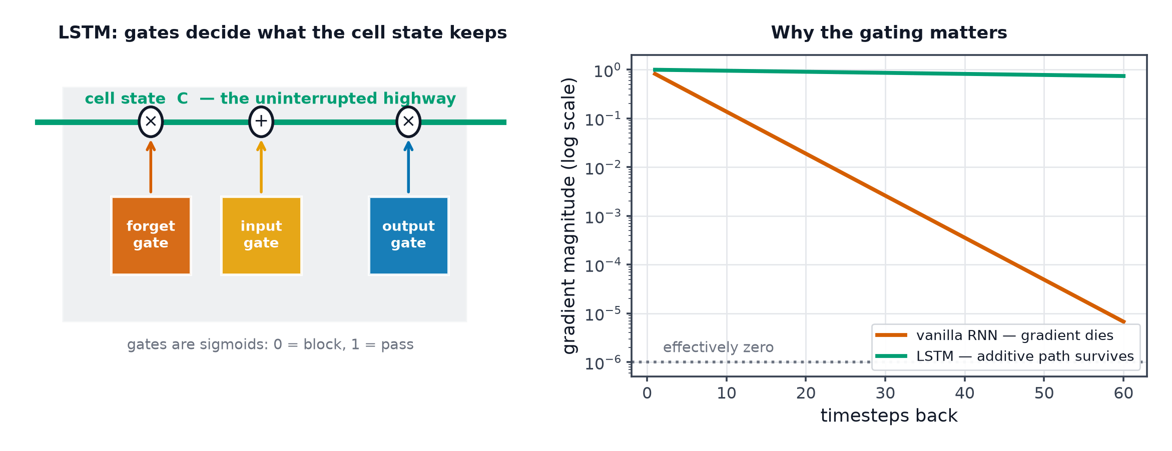
An additive cell state with multiplicative gates gives gradients a highway through time, the same trick residual connections use through depth.

The cell state runs across the top almost untouched — information passes along it by addition rather than repeated multiplication. That additive path is what keeps the gradient alive over long spans, as the right panel shows.

The problem, restated

A plain RNN's hidden state is overwritten at every step — $h_t$ depends on $h_{t-1}$ only through a repeated matrix multiplication and squashing non-linearity, exactly the multiplicative chain that vanishes across many steps.

The cell state as a conveyor belt

LSTM introduces a second state, the cell state $c_t$, updated additively rather than through a repeated matrix multiplication — information can flow along the cell state largely unchanged across many timesteps, only modified where a gate explicitly decides to add or remove something.

The forget gate

$$f_t = \sigma(W_f [h_{t-1}, x_t] + b_f)$$

A sigmoid output between 0 and 1, per cell-state dimension, deciding how much of the previous cell state to keep ($f_t \approx 1$: keep it; $f_t \approx 0$: discard it).

The input gate and the candidate

$$i_t = \sigma(W_i [h_{t-1}, x_t] + b_i), \qquad \tilde c_t = \tanh(W_c [h_{t-1}, x_t] + b_c)$$

$i_t$ decides how much of the new candidate information $\tilde c_t$ to write into the cell state.

The output gate

$$o_t = \sigma(W_o [h_{t-1}, x_t] + b_o)$$

Decides how much of the (updated) cell state to expose as the hidden state output.

The full LSTM forward pass

$$c_t = f_t \odot c_{t-1} + i_t \odot \tilde c_t, \qquad h_t = o_t \odot \tanh(c_t)$$

Symbol	Meaning
$c_t$	cell state — the additive, long-term memory path
$h_t$	hidden state — the gated, per-step output
$f_t, i_t, o_t$	forget, input, output gates (each a sigmoid, values in $[0,1]$)
$\tilde c_t$	candidate new information, proposed at this timestep

In words: the forget gate decides what to erase from long-term memory, the input gate decides what new information to write in, and the output gate decides what part of memory to actually reveal as this step's output — three separate, learned decisions, rather than one uncontrolled overwrite.

Why the additive cell update prevents vanishing

$$\frac{\partial c_t}{\partial c_{t-1}} = f_t$$

Unlike the plain RNN's repeated matrix multiplication, the cell-state gradient path is a simple elementwise multiplication by the forget gate — if $f_t$ stays close to 1 (the gate has learned "keep this information"), gradients can flow across many timesteps largely undiminished, exactly analogous to Skip Connections and Depth's "+1" identity term, except here the identity path is gated rather than fixed.

The GRU: reset and update gates, fewer parameters

The Gated Recurrent Unit simplifies LSTM's three gates and two states down to two gates and one state — a reset gate (how much past state to ignore when computing the candidate) and an update gate (how much to blend the candidate into the new state), with no separate cell state at all. Fewer parameters per cell than LSTM, for a comparable qualitative fix to the vanishing-gradient problem.

LSTM vs. GRU: the honest verdict

Empirically, the two perform comparably across most tasks — neither reliably and substantially outperforms the other, so the choice often comes down to GRU's smaller parameter count and slightly faster training versus LSTM's somewhat more expressive three-gate structure, rather than any decisive quality difference.

Peephole and other variants, briefly

Peephole connections let the gates see the cell state directly (not just the previous hidden state) when computing their values — one of many published LSTM variants, generally producing only marginal, task-dependent differences from the standard formulation above.

What LSTMs were state of the art for

Machine translation, speech recognition, and most sequence modelling tasks throughout the mid-2010s, until Transformer Architecture displaced them across nearly all of these applications within a few years of its publication.

Why transformers displaced them, and where LSTMs still make sense

Transformers parallelise across the whole sequence during training (no sequential dependency to wait on) and handle long-range dependencies via direct attention rather than a gated relay through many timesteps. LSTMs/GRUs still make sense for: small datasets (transformers' lack of a built-in sequential inductive bias means they typically need more data to reach comparable performance), genuinely streaming/online applications (an RNN naturally processes one step at a time with $O(1)$ state, while a transformer's attention mechanism looks back over the full context), and resource-constrained/tiny-device deployment where a transformer's quadratic attention cost is prohibitive.

Code: LSTM cell forward pass showing gate activity, PyTorch comparison

lstm_demo.py

import numpy as np
import torch
import torch.nn as nn

def sigmoid(z): return 1 / (1 + np.exp(-z))

class LSTMCellFromScratch:
    def __init__(self, input_dim, hidden_dim, rng):
        concat_dim = input_dim + hidden_dim
        self.Wf = rng.normal(scale=0.1, size=(hidden_dim, concat_dim))
        self.Wi = rng.normal(scale=0.1, size=(hidden_dim, concat_dim))
        self.Wc = rng.normal(scale=0.1, size=(hidden_dim, concat_dim))
        self.Wo = rng.normal(scale=0.1, size=(hidden_dim, concat_dim))
        self.hidden_dim = hidden_dim

    def forward(self, x, h_prev, c_prev):
        concat = np.concatenate([h_prev, x])
        f = sigmoid(self.Wf @ concat)
        i = sigmoid(self.Wi @ concat)
        c_candidate = np.tanh(self.Wc @ concat)
        o = sigmoid(self.Wo @ concat)
        c = f * c_prev + i * c_candidate
        h = o * np.tanh(c)
        return h, c, {"forget_gate": f, "input_gate": i, "output_gate": o}

rng = np.random.default_rng(0)
cell = LSTMCellFromScratch(input_dim=5, hidden_dim=8, rng=rng)
h, c = np.zeros(8), np.zeros(8)
X = rng.normal(size=(10, 5))

print("step | mean forget gate | mean input gate | mean output gate")
for t, x_t in enumerate(X):
    h, c, gates = cell.forward(x_t, h, c)
    print(f"{t:4d} | {gates['forget_gate'].mean():.3f}          | {gates['input_gate'].mean():.3f}"
          f"          | {gates['output_gate'].mean():.3f}")

# --- PyTorch LSTM vs RNN, sequence classification ---
torch.manual_seed(0)
X_torch = torch.randn(32, 20, 5)  # batch, seq_len, input_dim
y_torch = (X_torch.sum(dim=(1, 2)) > 0).long()

for name, rnn_layer in [("nn.RNN", nn.RNN(5, 16, batch_first=True)),
                          ("nn.LSTM", nn.LSTM(5, 16, batch_first=True))]:
    classifier = nn.Sequential(nn.Linear(16, 2))
    optimizer = torch.optim.Adam(list(rnn_layer.parameters()) + list(classifier.parameters()), lr=0.01)
    for step in range(100):
        optimizer.zero_grad()
        output, _ = rnn_layer(X_torch)
        logits = classifier(output[:, -1, :])  # use the final timestep's hidden state
        loss = nn.functional.cross_entropy(logits, y_torch)
        loss.backward()
        optimizer.step()
    print(f"{name} final training loss: {loss.item():.4f}")

See also

• Recurrent Neural Networks — the vanishing-gradient problem this architecture directly fixes.
• Seq2Seq and Encoder-Decoder — LSTM/GRU cells as the standard building block of early translation architectures.