Parameter-Efficient Finetuning

Full fine-tuning of a seven-billion-parameter model requires storing gradients and Adam's two moment buffers for every single one of those parameters — memory that a single consumer GPU simply doesn't have. Parameter-efficient fine-tuning methods sidestep this by training a tiny fraction of parameters instead, built on a striking empirical observation: the weight updates that fine-tuning actually needs are far lower-rank than the weight matrices themselves.

Key idea

Weight updates during fine-tuning are low-rank in practice, so you can train a small factorisation of the update instead of the weights themselves.

LoRA freezes the pretrained matrix and trains a low-rank update beside it. At rank 8 that is roughly 0.4 % of the original parameter count — and because the product merges back at inference, it costs no extra latency.

Why full fine-tuning is expensive

For a model with $P$ parameters trained with Adam, GPU Training and Mixed Precision already established roughly $4P$ values are needed just for optimiser state (parameters, gradients, two moment buffers) — for a 7B model, this alone requires tens of gigabytes, before counting activations.

The low-rank hypothesis

Empirically, the change in weights during fine-tuning ($\Delta W = W_{\text{finetuned}} - W_{\text{pretrained}}$) tends to have much lower effective rank than the full weight matrix $W$ itself — the fine-tuned task doesn't need to reach every possible direction in weight space, only a comparatively small subspace of it.

LoRA: the B·A decomposition

$$W' = W + BA, \qquad B \in \mathbb{R}^{d \times r}, \; A \in \mathbb{R}^{r \times k}, \; r \ll \min(d, k)$$

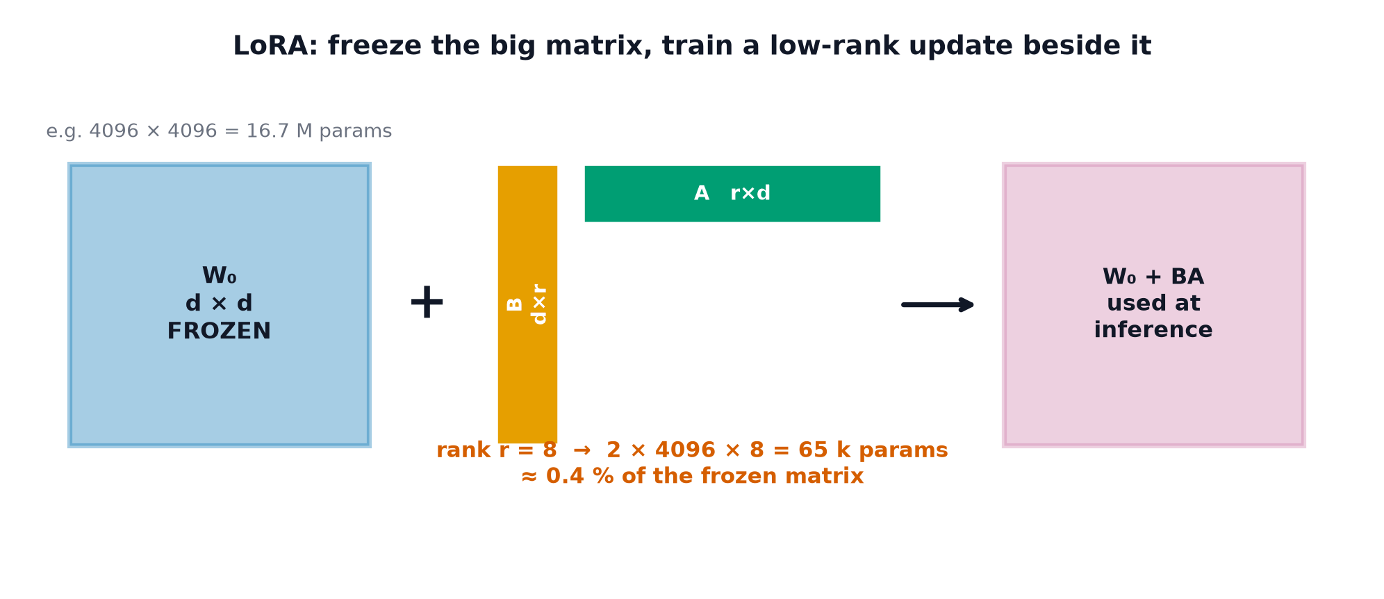
The original weight matrix $W$ (dimensions $d \times k$) stays entirely frozen. A new, much smaller pair of matrices $B$ and $A$, with a small inner rank $r$, is trained instead — their product $BA$ approximates the low-rank update $\Delta W$ the low-rank hypothesis predicts should suffice.

Rank r and alpha

$r$ (typically 4–64) directly controls the trade-off: larger $r$ gives more expressive updates at the cost of more trainable parameters. A scaling factor $\alpha/r$ multiplies the $BA$ product before adding it to $W$, controlling how strongly the LoRA update influences the frozen base weights relative to their original magnitude.

Symbol	Meaning
$W$	the frozen pretrained weight matrix
$B, A$	the trainable low-rank factors
$r$	LoRA rank — the inner dimension of the factorisation
$\alpha$	scaling factor, applied as $\alpha/r$

Which modules to target

LoRA is typically applied to the query and value projection matrices within attention layers (Self-Attention in Depth) rather than every weight matrix in the model — empirically, these projections capture most of the benefit, and targeting a subset keeps the trainable parameter count small.

Merging adapters back for zero inference overhead

Because $W' = W + BA$ is just an addition, once training finishes, $B$ and $A$ can be multiplied together and added directly into $W$, producing a single merged weight matrix — at inference time, there's no separate LoRA computation at all, and no latency overhead relative to a fully fine-tuned model of the same architecture.

Serving many adapters over one base model

Because LoRA's trained parameters ($B, A$) are tiny relative to the full model, many different task-specific adapters can be stored cheaply and swapped in against the same frozen base model at serving time — a substantial memory saving versus hosting a fully separate fine-tuned copy of the base model per task.

QLoRA: 4-bit base weights, NF4, double quantisation

Combines LoRA with aggressive quantisation of the frozen base model: weights are stored in 4-bit precision using NF4 (a data type designed to match the actual statistical distribution of neural network weights, rather than a generic uniform 4-bit encoding), and double quantisation additionally quantises the quantisation constants themselves for further memory savings. Paged optimizers use CPU memory as overflow for optimizer state during occasional memory spikes, preventing an out-of-memory crash rather than requiring the entire training run to fit in GPU memory at all times. Together, these let a model far too large to fully fine-tune on a given GPU be fine-tuned via LoRA on that same GPU.

Adapters, prefix tuning, prompt tuning, IA³

Adapters: insert small trainable bottleneck layers between existing frozen layers, rather than modifying existing weights at all. Prefix tuning: prepend a small number of trainable "virtual token" vectors to the input at every layer, steering the frozen model's behaviour without touching its weights. Prompt tuning: similar, but only at the input embedding layer, not every layer. IA³: learns a small set of per-channel rescaling vectors applied to existing activations — each represents a different point on the trainable-parameter-count vs. expressiveness trade-off from LoRA.

Comparison table

Method	Trainable parameters	Memory	Quality gap vs. full fine-tune	Inference cost
Full fine-tuning	100%	highest	none (baseline)	baseline
LoRA	typically under 1%	low	small to negligible	zero, once merged
QLoRA	typically under 1%	lowest	small to negligible	zero, once merged and dequantised
Prompt/prefix tuning	very small	low	often larger, task-dependent	small ongoing overhead

When full fine-tuning is still the right answer

When the fine-tuning task differs substantially from anything in pretraining (requiring the model to learn genuinely new structure, not just adapt existing capability), when compute and memory aren't binding constraints, or when squeezing out the absolute maximum quality matters more than efficiency — full fine-tuning remains the strongest option when its cost is affordable.

Code: a LoRA layer from scratch, parameter counts, verified merge

lora_demo.py

import torch
import torch.nn as nn

class LoRALinear(nn.Module):
    def __init__(self, base_linear, rank=4, alpha=8):
        super().__init__()
        self.base = base_linear
        for p in self.base.parameters():
            p.requires_grad = False  # frozen base weights
        d_out, d_in = base_linear.weight.shape
        self.A = nn.Parameter(torch.randn(rank, d_in) * 0.01)
        self.B = nn.Parameter(torch.zeros(d_out, rank))  # zero init: LoRA starts as a no-op
        self.scaling = alpha / rank

    def forward(self, x):
        return self.base(x) + (x @ self.A.T @ self.B.T) * self.scaling

    def merged_weight(self):
        return self.base.weight + (self.B @ self.A) * self.scaling

torch.manual_seed(0)
base_layer = nn.Linear(512, 512)
lora_layer = LoRALinear(base_layer, rank=8)

full_params = sum(p.numel() for p in base_layer.parameters())
lora_params = sum(p.numel() for p in [lora_layer.A, lora_layer.B])
print(f"full fine-tuning would train: {full_params:,} parameters")
print(f"LoRA trains only:             {lora_params:,} parameters ({100*lora_params/full_params:.2f}%)")

# --- Train the LoRA adapter briefly, then verify the merge produces identical outputs ---
optimizer = torch.optim.Adam([lora_layer.A, lora_layer.B], lr=0.01)
x = torch.randn(16, 512)
target = torch.randn(16, 512)
for _ in range(50):
    optimizer.zero_grad()
    loss = ((lora_layer(x) - target) ** 2).mean()
    loss.backward()
    optimizer.step()

merged = nn.Linear(512, 512)
merged.weight.data = lora_layer.merged_weight()
merged.bias.data = base_layer.bias.data

lora_output = lora_layer(x)
merged_output = merged(x)
print("max difference between LoRA and merged outputs:", (lora_output - merged_output).abs().max().item())

See also

• Finetuning and Instruction Tuning — the full fine-tuning process this page makes affordable for large models.
• GPU Training and Mixed Precision — the memory accounting that motivates parameter-efficient methods.