Recurrent Neural Networks

Every network up to this point has processed a single fixed-size input. Language, audio, and time series don't come in fixed sizes — a sentence can be five words or fifty. Recurrent networks were the first architecture built specifically to handle that: reuse the same weights at every timestep, carrying a hidden state forward as a compressed summary of everything seen so far.

Key idea

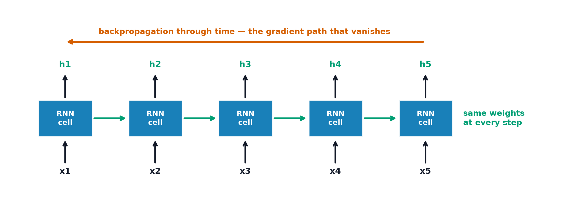
An RNN reuses one weight matrix at every timestep, which gives it unbounded context in principle and a vanishing gradient in practice.

Unrolled, an RNN is a very deep network that reuses one weight matrix at every step. The red path is backpropagation through time — and repeatedly multiplying by the same matrix is precisely why the gradient vanishes or explodes.

Why feedforward networks cannot handle variable length

An MLP's input layer has a fixed number of units — there's no natural way to feed it a 5-word sentence one moment and a 50-word sentence the next without padding to some fixed maximum (wasteful) or truncating (lossy). RNNs sidestep this by processing one token at a time, regardless of sequence length.

The recurrence relation

$$h_t = \tanh(W_{hh} h_{t-1} + W_{xh} x_t + b)$$

At every timestep, combine the current input $x_t$ with the previous hidden state $h_{t-1}$ using the same weight matrices, producing a new hidden state $h_t$.

The hidden state as compressed history

$h_t$ is meant to summarise everything relevant from $x_1, \ldots, x_t$ in a single fixed-size vector — an RNN's entire "memory" of the sequence so far is squeezed through this one vector at every step, which is both the mechanism that makes variable-length processing possible and (as covered below) the mechanism that ultimately limits it.

Unrolling through time

Although the recurrence is defined step-by-step, an RNN processing a sequence of length $T$ can be "unrolled" into an equivalent feedforward computation graph with $T$ layers, each sharing identical weights — this unrolled view is exactly what Backpropagation is applied to.

Backpropagation through time (BPTT)

Backpropagation applied to the unrolled graph, computing gradients with respect to the shared weight matrices by summing their contribution across every timestep they were used at. Truncated BPTT limits how far back gradients are propagated (e.g. only the last 50 steps), trading some long-range gradient accuracy for tractable memory and compute cost on very long sequences.

Parameter sharing across timesteps

The same $W_{hh}, W_{xh}$ are reused at every single timestep — this is what lets an RNN generalise to sequences of any length with a fixed parameter count, but it's also exactly the condition Vanishing and Exploding Gradients identified as most severe: the same matrix, multiplied against itself repeatedly.

The vanishing gradient in the recurrent case, derived

$$\frac{\partial h_T}{\partial h_1} = \prod_{t=2}^T \frac{\partial h_t}{\partial h_{t-1}} = \prod_{t=2}^T W_{hh}^\top \text{diag}(\tanh'(z_t))$$

Symbol	Meaning
$h_t$	hidden state at timestep $t$
$W_{hh}, W_{xh}$	recurrent and input weight matrices, shared across all timesteps
$T$	sequence length

This product involves the identical $W_{hh}$ repeated $T-1$ times — for sequences of any real length, this is exactly the pathological case Vanishing and Exploding Gradients described: unlike a feedforward network where different layers might have different weight scales that partially compensate for each other, here every factor is literally the same matrix, so any deviation of its spectral radius from 1 compounds relentlessly.

Sequence-to-one, sequence-to-sequence, one-to-sequence

Sequence-to-one: consume a whole sequence, produce one output at the end (e.g. sentiment classification). Sequence-to-sequence: consume a sequence, produce another sequence, often of different length (translation — see Seq2Seq and Encoder-Decoder). One-to-sequence: consume a single input, generate a sequence (e.g. image captioning).

Bidirectional RNNs and their streaming cost

A bidirectional RNN runs two RNNs over the sequence, one forward and one backward, concatenating their hidden states — captures context from both directions at every position, at the direct cost that it requires seeing the entire sequence before producing any output, ruling it out for streaming or real-time generation tasks where future tokens aren't available yet.

Stacked RNNs

Stacking multiple RNN layers (feeding the hidden-state sequence of one layer as the input sequence to the next) increases representational capacity, analogous to depth in a feedforward network — with the same Vanishing and Exploding Gradients considerations compounding across both time and depth.

Why RNNs lost to transformers

Beyond the gradient issues, RNNs have a structural disadvantage that no amount of gating (see LSTM and GRU) fixes: computing $h_t$ requires $h_{t-1}$ to already exist — the recurrence is inherently sequential, and cannot be parallelised across timesteps the way Self-Attention in Depth's per-position computation can. On modern parallel hardware, this sequential dependency is a severe practical bottleneck that transformers were specifically designed to remove.

Code: RNN cell forward/BPTT from scratch, gradient norms vanishing, PyTorch comparison

rnn_demo.py

import numpy as np
import torch
import torch.nn as nn

def rnn_forward(X, Whh, Wxh, b):
    T, input_dim = X.shape
    hidden_dim = Whh.shape[0]
    h = np.zeros(hidden_dim)
    hidden_states = [h]
    for t in range(T):
        h = np.tanh(Whh @ h + Wxh @ X[t] + b)
        hidden_states.append(h)
    return hidden_states

def rnn_bptt_gradient_norms(hidden_states, Whh):
    """Trace ||dh_T/dh_t|| back through time to show the vanishing effect."""
    T = len(hidden_states) - 1
    grad = np.eye(Whh.shape[0])
    norms = []
    for t in reversed(range(1, T + 1)):
        deriv = 1 - hidden_states[t] ** 2  # tanh'(z) in terms of h = tanh(z)
        grad = (Whh.T * deriv) @ grad
        norms.append(np.linalg.norm(grad))
    return list(reversed(norms))

rng = np.random.default_rng(0)
seq_len, hidden_dim, input_dim = 50, 20, 5
Whh = rng.normal(scale=0.9, size=(hidden_dim, hidden_dim)) / np.sqrt(hidden_dim)  # spectral radius < 1
Wxh = rng.normal(scale=0.5, size=(hidden_dim, input_dim))
b = np.zeros(hidden_dim)
X = rng.normal(size=(seq_len, input_dim))

hidden_states = rnn_forward(X, Whh, Wxh, b)
grad_norms = rnn_bptt_gradient_norms(hidden_states, Whh)
print("gradient norm at t=1 (earliest):", grad_norms[0])
print("gradient norm at t=45 (near the end):", grad_norms[44])
print("ratio (vanishing across 45 steps):", grad_norms[44] / grad_norms[0])

# --- PyTorch nn.RNN, for comparison ---
torch.manual_seed(0)
rnn = nn.RNN(input_size=input_dim, hidden_size=hidden_dim, batch_first=True)
X_torch = torch.tensor(X, dtype=torch.float32).unsqueeze(0)  # add batch dimension
output, h_n = rnn(X_torch)
print("\nPyTorch RNN output shape:", output.shape, " final hidden state shape:", h_n.shape)

See also

• Vanishing and Exploding Gradients — the general theory this page's derivation instantiates for the recurrent case.
• LSTM and GRU — the gated architecture that kept recurrent networks trainable for two more decades.