Self-Attention in Depth

Self-attention consumes more of a transformer's compute than any other single operation, and its exact mechanics — how heads split the embedding, how masking works, how memory scales — decide almost everything about a model's practical cost, from training time to how long a context window is affordable to serve.

Key idea

Multiple heads let the model attend to several kinds of relationship at once, at no extra cost, by splitting the same embedding across subspaces.

Queries and keys produce the scores; values carry the content that gets mixed. The √d divisor keeps the dot products from growing with dimension and driving the softmax into a near-one-hot regime where gradients vanish.

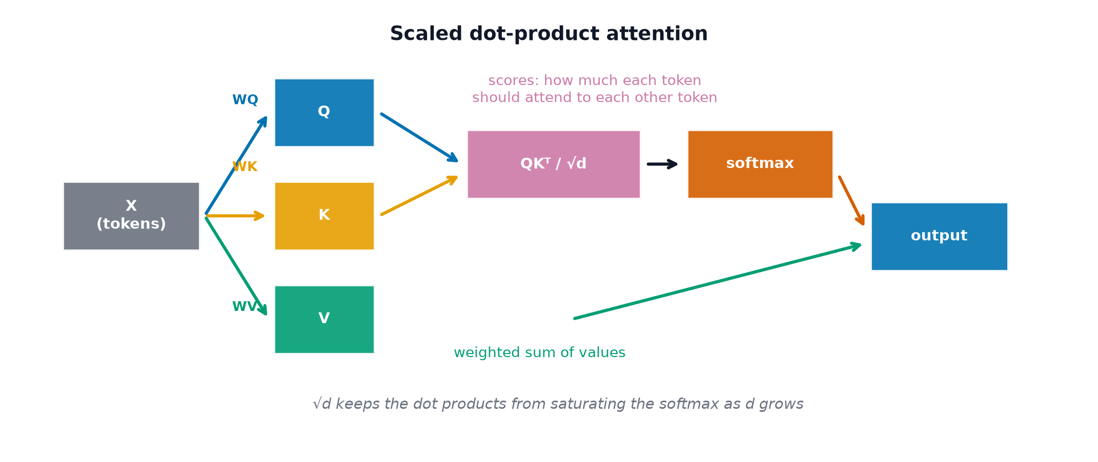
The Q/K/V projections and their shapes

From the same input $x \in \mathbb{R}^{n \times d}$, three learned linear projections produce $Q = xW_Q$, $K = xW_K$, $V = xW_V$, each typically shape $(n, d)$ — self-attention because all three come from the same sequence, not from separate encoder/decoder inputs.

Multi-head attention: split, attend, concatenate, project

Rather than one attention computation over the full $d$-dimensional embedding, split $Q, K, V$ into $h$ heads, each of dimension $d_k = d/h$; run scaled dot-product attention independently within each head; concatenate all heads' outputs back together; apply one final linear projection $W_O$.

$$\text{MultiHead}(Q,K,V) = \text{Concat}(\text{head}_1, \ldots, \text{head}_h)W_O, \quad \text{head}_i = \text{Attention}(QW_i^Q, KW_i^K, VW_i^V)$$

Why heads are cheaper than they look

Each head operates on a $d/h$-dimensional slice of the embedding, not a full $d$-dimensional copy — the total compute and parameter count across all $h$ heads combined is comparable to running a single full-dimension attention once, not $h$ times the cost. Splitting is what lets multiple heads exist at essentially the cost of one.

What different heads empirically learn

Analyses of trained transformers have found individual heads specialising in identifiable patterns — some attend predominantly to adjacent positions, some to specific syntactic relationships (a verb attending to its subject), some to rare or unusual tokens. The caveat: these findings vary across models, layers, and training runs, and not every head has a clean, human-interpretable specialisation — treat per-head interpretability claims as suggestive evidence, not a settled mechanistic account.

Symbol	Meaning
$h$	number of attention heads
$d_k = d/h$	dimensionality per head
$W_Q, W_K, W_V, W_O$	the four learned projection matrices

The causal mask, implemented

Before the softmax, add $-\infty$ (in practice, a very large negative number) to every score at a position $j > i$ for query position $i$ — after softmax, those positions receive exactly zero weight, enforcing the autoregressive constraint from Transformer Architecture.

Padding masks, and the bug when you forget one

When batching sequences of different lengths, shorter sequences are padded to a common length — without an explicit padding mask, the model attends to (and is influenced by) meaningless padding tokens as if they were real content, silently corrupting every prediction in a batch with variable-length sequences. This is a common, easy-to-miss bug distinct from the causal mask, and both are frequently required simultaneously in decoder training.

Attention as a graph operation

Self-attention can be viewed as computing, for every pair of positions, an edge weight in a fully-connected graph over the sequence — unlike a CNN's fixed local connectivity or an RNN's fixed sequential connectivity, attention's connectivity pattern is entirely learned and can, in principle, connect any two positions directly regardless of their distance in the sequence.

The O(n²) memory problem

Attention is O(n²) in sequence length while the feed-forward layers are linear. Below a few thousand tokens the MLPs dominate the cost; past that, attention takes over — which is what every long-context method is trying to fix.

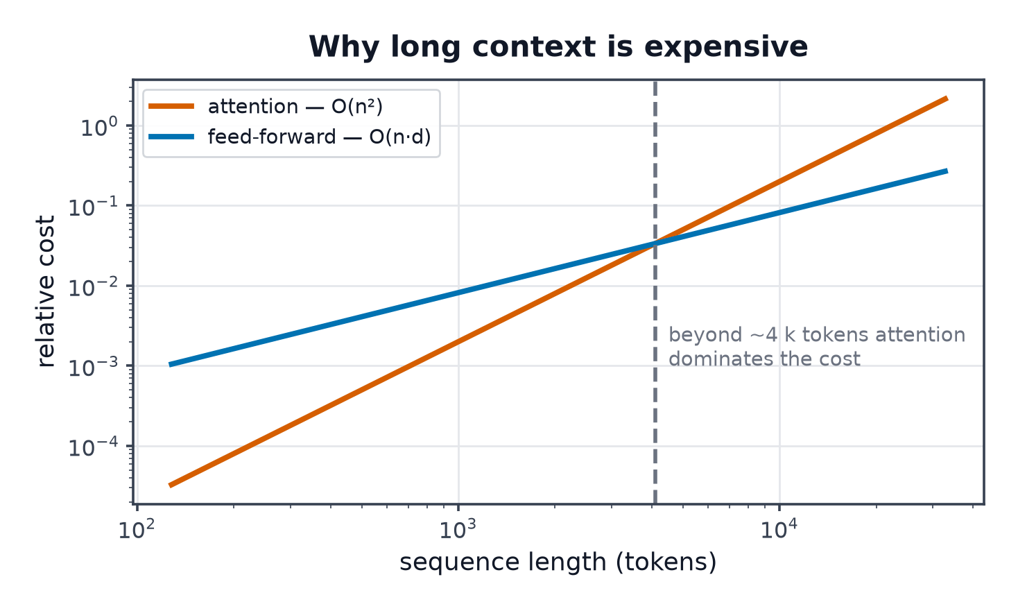
Storing the full attention weight matrix requires $O(n^2)$ memory per head, per layer — for long sequences, this becomes the dominant memory cost, often exceeding the memory used by the model's parameters themselves.

KV caching at inference

During autoregressive generation, each new token's query only needs to attend to all previous tokens' keys and values — which don't change as generation proceeds. Caching these keys and values (rather than recomputing them from scratch at every generation step) turns each new token's generation cost from $O(n)$ (recomputing everything) down to $O(1)$ additional work per step, at the cost of memory proportional to sequence length times model size to store the cache.

$$\text{KV cache size} \approx 2 \times n \times d \times N_{\text{layers}} \times \text{bytes per value}$$

Efficiency variants: sparse, linear, sliding-window attention

Sparse attention: restrict each position to attend only to a fixed subset of others (not the full $n$), trading some modelling flexibility for sub-quadratic cost. Linear attention: reformulate the attention computation to avoid ever materialising the full $n \times n$ score matrix, achieving linear rather than quadratic scaling, generally at some cost to modelling quality. Sliding-window attention: each position attends only within a fixed-size local window — cheap, and effective when most relevant context is genuinely local.

FlashAttention: exact, not approximate

An important distinction from the variants above: FlashAttention computes the exact same attention output as standard scaled dot-product attention — it's an IO-aware implementation, reordering and fusing the computation to minimise slow memory (GPU HBM) reads/writes rather than fast on-chip memory operations, achieving substantial real-world speedups and memory savings without any approximation or quality trade-off.

Multi-query and grouped-query attention

Multi-query attention: share a single set of keys/values across all query heads (instead of each head having its own K/V projection) — dramatically shrinks the KV cache size, at some cost to model quality. Grouped-query attention: a middle ground, sharing K/V across small groups of query heads rather than either fully separate (standard multi-head) or fully shared (multi-query) — driven directly by the KV cache memory and inference-latency concerns identified above, not by training-time considerations.

Code: multi-head attention from scratch, per-head heatmaps, KV cache timing

self_attention_depth_demo.py

import numpy as np
import torch
import torch.nn as nn
import time

def softmax(z, axis=-1):
    exp = np.exp(z - z.max(axis=axis, keepdims=True))
    return exp / exp.sum(axis=axis, keepdims=True)

def multi_head_attention(x, Wq, Wk, Wv, Wo, n_heads):
    n, d = x.shape
    d_k = d // n_heads
    Q, K, V = x @ Wq, x @ Wk, x @ Wv
    Q, K, V = (t.reshape(n, n_heads, d_k).transpose(1, 0, 2) for t in (Q, K, V))
    head_outputs = []
    for h in range(n_heads):
        scores = Q[h] @ K[h].T / np.sqrt(d_k)
        weights = softmax(scores)
        head_outputs.append(weights @ V[h])
    concatenated = np.concatenate(head_outputs, axis=-1)
    return concatenated @ Wo, np.stack([softmax(Q[h] @ K[h].T / np.sqrt(d_k)) for h in range(n_heads)])

rng = np.random.default_rng(0)
n, d, n_heads = 6, 16, 4
x = rng.normal(size=(n, d))
Wq, Wk, Wv, Wo = (rng.normal(scale=0.1, size=(d, d)) for _ in range(4))
output, per_head_weights = multi_head_attention(x, Wq, Wk, Wv, Wo, n_heads)
print("output shape:", output.shape, " per-head attention shape:", per_head_weights.shape)
for h in range(n_heads):
    print(f"head {h} attention row sums:", per_head_weights[h].sum(axis=1).round(3))

# --- KV cache timing: recompute-everything vs. cached generation ---
d_model, n_layers = 64, 4
mha = nn.MultiheadAttention(d_model, num_heads=8, batch_first=True)

def generate_no_cache(n_steps):
    seq = torch.randn(1, 1, d_model)
    for _ in range(n_steps):
        out, _ = mha(seq, seq, seq)  # recomputes attention over the WHOLE growing sequence each step
        seq = torch.cat([seq, out[:, -1:, :]], dim=1)

start = time.perf_counter()
generate_no_cache(30)
print(f"\nno-cache generation (30 steps): {time.perf_counter() - start:.4f}s"
      " -- cost grows with sequence length at every step, exactly what KV caching avoids")

See also

• Transformer Architecture — where multi-head attention sits within the full encoder/decoder stack.
• Positional Encodings — the missing ingredient attention alone cannot supply.