Word Embeddings

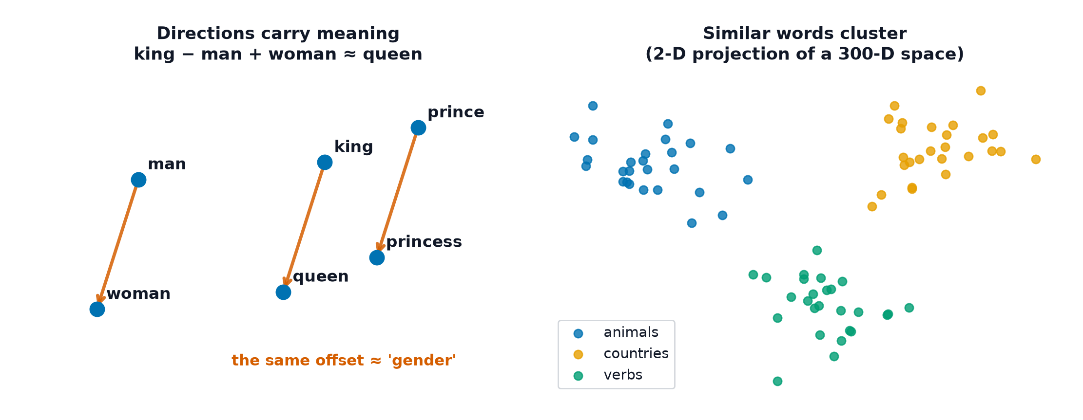
One-hot encoding a vocabulary treats every word as equally different from every other word — "cat" is exactly as far from "dog" as it is from "bicycle." Word embeddings replace that with geometry: words that appear in similar contexts end up close together in a continuous vector space, and "close" starts to mean "similar" in a way a model can actually use.

Key idea

A word's meaning is approximated by the company it keeps — embeddings are the numerical form of that assumption.

Embeddings place words so that geometry carries meaning: the offset from *king* to *queen* is roughly the offset from *man* to *woman*. Similar words cluster, which is what makes nearest-neighbour retrieval over embeddings work.

One-hot encoding and why it carries no similarity

Representing each word as a vector with a single 1 and zeros elsewhere gives every pair of distinct words an identical Euclidean distance and a dot product of exactly zero — the representation is correct as an identifier but carries no information about meaning or relatedness at all.

The distributional hypothesis

"You shall know a word by the company it keeps" — the linguistic principle that words appearing in similar contexts tend to have similar meanings. Every method on this page operationalises this hypothesis in some form.

Count-based methods

Build a co-occurrence matrix (how often word $i$ appears near word $j$ across a corpus), then apply PPMI (positive pointwise mutual information, which reweights raw counts to downweight extremely common words) and LSA (latent semantic analysis — factorise the resulting matrix via SVD, the same machinery as PCA and SVD) to produce dense, lower-dimensional word vectors.

Word2Vec: skip-gram and CBOW

Skip-gram: given a centre word, predict the surrounding context words. CBOW (continuous bag of words): given the surrounding context words, predict the centre word — the reverse prediction direction of skip-gram. Both train a shallow neural network, and the learned weight matrix itself (not the prediction task's output) becomes the word embedding table — the prediction task is a means to an end, not the goal.

Negative sampling

Training skip-gram's full softmax over the entire vocabulary at every step is prohibitively expensive for a vocabulary of hundreds of thousands of words. Negative sampling reframes it as a binary classification problem: for each true (centre, context) pair, also sample a handful of random, likely-incorrect (centre, random-word) pairs, and train the model to distinguish real pairs from these negative samples — dramatically cheaper per step, and empirically works about as well as the full softmax for the embeddings' downstream quality.

$$L = -\log\sigma(v_c \cdot v_o) - \sum_{i=1}^k \mathbb{E}_{w_i \sim P_n}\big[\log\sigma(-v_c \cdot v_{w_i})\big]$$

Symbol	Meaning
$v_c, v_o$	embedding vectors for the centre word and a true context word
$k$	number of negative samples per true pair
$P_n$	the noise distribution negative samples are drawn from

GloVe

Rather than word2vec's local-window prediction task, GloVe factorises global co-occurrence statistics directly, explicitly targeting the property that ratios of co-occurrence probabilities encode meaningful relationships — a different training objective converging on embeddings with broadly similar practical quality to word2vec.

FastText and subword vectors

Represents each word as the sum of embeddings for its character n-grams (e.g. "apple" decomposes into <ap, app, ppl, ple, le> plus the whole word) — this lets FastText produce a reasonable embedding for a word it never saw during training, as long as it shares subword pieces with words it did see, directly addressing word2vec/GloVe's inability to embed out-of-vocabulary words at all.

The analogy arithmetic result, and its critiques

The famous example: $\text{vec("king")} - \text{vec("man")} + \text{vec("woman")} \approx \text{vec("queen")}$ — vector arithmetic on embeddings capturing a semantic relationship. Honest critique: this result is considerably less robust than the original demonstrations suggested, working reliably only for a curated subset of relationships and word pairs, and the search procedure used to find the "nearest" analogy answer subtly excludes the input words themselves, which inflates apparent accuracy.

Cosine similarity as the standard measure

$$\text{sim}(u, v) = \frac{u \cdot v}{\|u\|\|v\|}$$

Measures the angle between two embedding vectors, ignoring magnitude — the standard similarity measure throughout NLP, because embedding direction tends to carry more semantic meaning than raw vector length.

Static vs. contextual embeddings

Word2vec/GloVe/FastText assign one fixed vector per word, regardless of context — "bank" gets the identical embedding whether it means a riverbank or a financial institution. BERT-style contextual embeddings (Transformer Variants) instead compute a different embedding for the same word depending on its surrounding sentence — a substantial capability jump, since word sense disambiguation requires exactly this context-sensitivity.

Sentence embeddings

Extending the idea from single words to whole sentences or documents — pooling contextual word embeddings, or training a model specifically to produce one vector per sentence such that similar-meaning sentences land close together, the foundation of semantic search and retrieval systems (see LangChain's embeddings material).

Bias encoded in embeddings

Embeddings trained on real-world text corpora reliably encode the biases present in that text — measurably, the same analogy-arithmetic technique that finds "king - man + woman ≈ queen" also finds occupation-gender associations reflecting historical societal bias in the training corpus, not any actual property of the occupations themselves. This is a direct, measurable consequence of the distributional hypothesis: embeddings capture what the text says, including its biases, not some bias-free ground truth.

Where embeddings are used today

Retrieval (finding semantically similar documents), clustering (grouping similar text), and as engineered features for downstream classical ML models — largely superseded, for direct language understanding tasks, by contextual embeddings produced as a byproduct of large pretrained transformer models.

Code: skip-gram with negative sampling from scratch, sentence embeddings compared

Outside the master library whitelist

The sentence-embedding block below uses sentence-transformers, not in the default library set. Install with pip install sentence-transformers.

word_embeddings_demo.py

import numpy as np

corpus = "the cat sat on the mat the dog sat on the rug the cat and dog are friends".split()
vocab = sorted(set(corpus))
word_to_idx = {w: i for i, w in enumerate(vocab)}
window = 2

pairs = []
for i, word in enumerate(corpus):
    for j in range(max(0, i-window), min(len(corpus), i+window+1)):
        if i != j:
            pairs.append((word_to_idx[word], word_to_idx[corpus[j]]))

rng = np.random.default_rng(0)
embed_dim, vocab_size = 10, len(vocab)
W_center = rng.normal(scale=0.1, size=(vocab_size, embed_dim))
W_context = rng.normal(scale=0.1, size=(vocab_size, embed_dim))

def sigmoid(z): return 1 / (1 + np.exp(-z))

lr = 0.05
for epoch in range(200):
    for center, context in pairs:
        neg_samples = rng.integers(0, vocab_size, size=3)
        v_c = W_center[center]
        pos_score = sigmoid(v_c @ W_context[context])
        grad_pos = (pos_score - 1)
        W_center[center] -= lr * grad_pos * W_context[context]
        W_context[context] -= lr * grad_pos * v_c
        for neg in neg_samples:
            neg_score = sigmoid(v_c @ W_context[neg])
            W_center[center] -= lr * neg_score * W_context[neg]
            W_context[neg] -= lr * neg_score * v_c

def nearest(word, k=3):
    v = W_center[word_to_idx[word]]
    sims = W_center @ v / (np.linalg.norm(W_center, axis=1) * np.linalg.norm(v) + 1e-8)
    return [vocab[i] for i in np.argsort(-sims)[1:k+1]]

print("nearest to 'cat':", nearest("cat"))
print("nearest to 'dog':", nearest("dog"))

# --- Real sentence embeddings, cosine similarity heatmap ---
from sentence_transformers import SentenceTransformer
model = SentenceTransformer("all-MiniLM-L6-v2")
sentences = ["The cat sat on the mat.", "A feline rested on the rug.", "The stock market fell today."]
embeddings = model.encode(sentences)
sims = embeddings @ embeddings.T / (np.linalg.norm(embeddings, axis=1)[:, None] * np.linalg.norm(embeddings, axis=1)[None, :])
print("\nsentence similarity matrix:\n", np.round(sims, 3))

See also

• Text Preprocessing and Tokenization — producing the tokens these embeddings represent.
• Manifold Learning — visualising a high-dimensional embedding space in 2-D.