Decomposition and Stationarity

Before fitting anything, split the series into the parts you can explain and the part you cannot. Decomposition does that; stationarity is the condition most classical models require before they will work at all.

Key idea

Decomposition separates trend, seasonality and residual so each can be handled on its own terms. Stationarity — constant mean, constant variance, constant autocorrelation — is what ARIMA and friends assume, and differencing plus a variance-stabilising transform is how you usually obtain it.

The same series viewed four ways. Once trend and seasonality are removed, what remains should look like structureless noise — if it does not, there is still signal on the table.

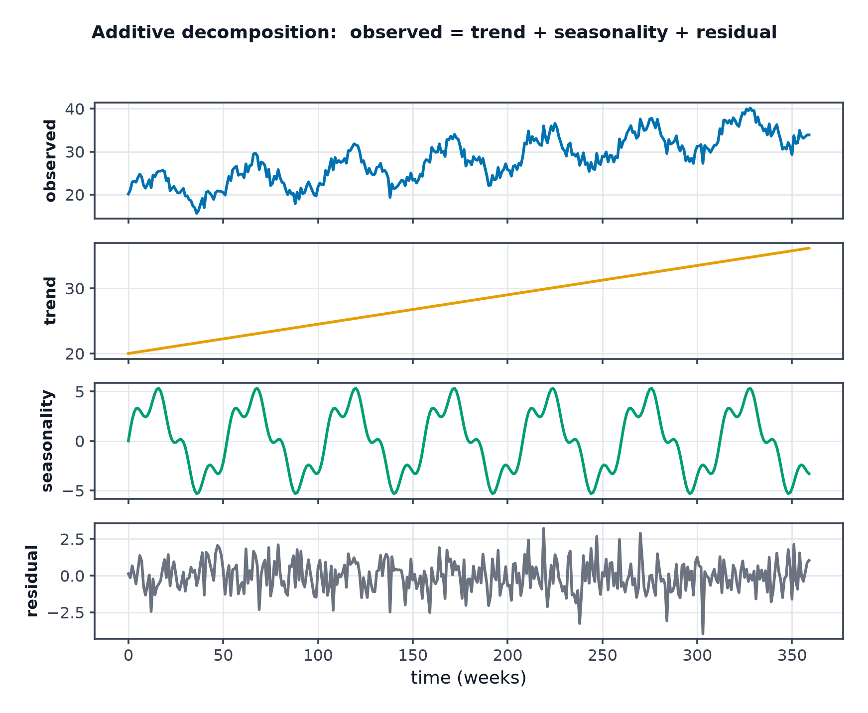
Additive or multiplicative

$$\text{additive:}\quad y_t = T_t + S_t + R_t \qquad\qquad \text{multiplicative:}\quad y_t = T_t \times S_t \times R_t$$

The choice is decided by looking at the series:

If the seasonal swing…	Use	Because
Stays the same absolute size as the level grows	Additive	The components genuinely add
Grows proportionally with the level	Multiplicative	The components scale together

Retail sales are almost always multiplicative — a December spike is +30 %, not +40,000 units, so it grows as the business does. Temperature is additive: summer is about 15 °C warmer than winter regardless of the decade.

Taking logs converts multiplicative into additive

$\log(T \times S \times R) = \log T + \log S + \log R$. This is why log-transforming is so common in forecasting: it turns proportional seasonality into constant seasonality, and simultaneously stabilises variance. It requires strictly positive data.

Methods, in increasing order of robustness

Method	Handles	Notes
Classical (moving-average)	Fixed seasonality	Simple, loses points at both ends
STL	Changing seasonality	Robust to outliers, the sensible default
X-13ARIMA-SEATS	Calendar effects, holidays	Official-statistics standard, heavy

STL (Seasonal-Trend decomposition using LOESS) is what to reach for unless you have a specific reason not to: it lets the seasonal pattern evolve over time and has a robust mode that stops a single spike distorting the whole decomposition.

Stationarity

A series is weakly stationary when three things hold for all $t$:

1. $\mathbb{E}[y_t] = \mu$ — constant mean
2. $\operatorname{Var}(y_t) = \sigma^2$ — constant variance
3. $\operatorname{Cov}(y_t, y_{t+k})$ depends only on $k$, not on $t$

The two ways stationarity usually fails. A drifting mean is fixed by differencing; a growing variance is fixed by a log or Box–Cox transform. Applying the wrong remedy leaves the problem in place.

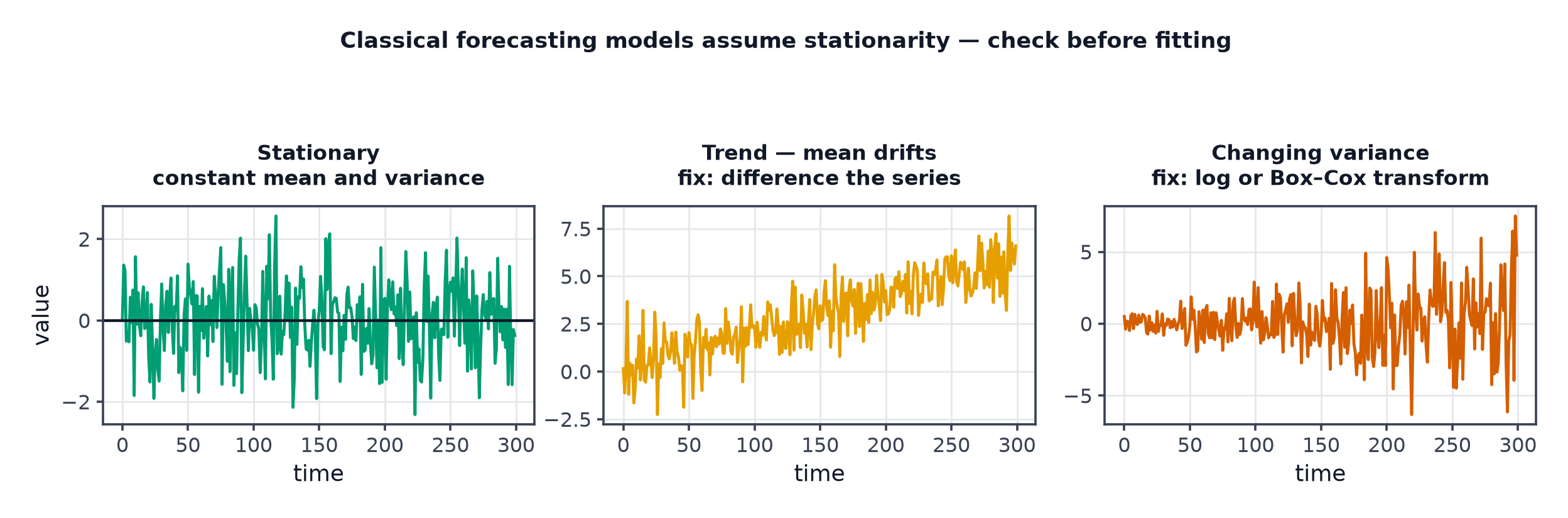
Note what stationarity does not mean: it does not mean the series is uninteresting or unpredictable. A stationary series can be strongly autocorrelated and highly forecastable. It only means the statistical rules generating it are stable.

Achieving it

Problem	Remedy
Trend (mean drifts)	First difference: $y'_t = y_t - y_{t-1}$
Seasonality	Seasonal difference: $y_t - y_{t-m}$ for period $m$
Growing variance	Log, square-root, or Box–Cox transform
Both trend and seasonality	Seasonal difference first, then check whether a first difference is still needed

Over-differencing is a real failure mode

Differencing an already-stationary series inflates its variance and injects artificial negative autocorrelation at lag 1, which then misleads your order selection. If the ACF after differencing drops sharply to a large negative value at lag 1, you have differenced once too often. Almost no real series needs $d > 2$.

Testing for it

Test	Null hypothesis	Reading it
ADF (Augmented Dickey–Fuller)	The series has a unit root (non-stationary)	Low p-value → stationary
KPSS	The series is stationary	Low p-value → non-stationary

The two nulls are opposite, which is exactly why they are used together. Agreement is decisive; disagreement usually means the series is fractionally integrated or has a structural break, and is a signal to look at the plot rather than the p-value.

Also: never rely on the test alone. Plot the series. A structural break — a pandemic, a pricing change, a sensor replacement — will fail every stationarity test while having nothing to do with trend, and no amount of differencing fixes it.

ACF and PACF: reading the correlation structure

Computed from 1,200 points of a simulated AR(2) process. The PACF is significant at lags 1 and 2 (+0.47, −0.36) and drops inside the confidence band from lag 3 onward — which is how the order is identified. The shaded band is the 95 % interval under the null of no correlation.

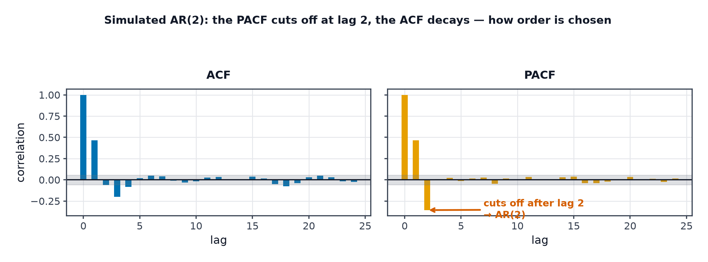
• ACF — correlation between $y_t$ and $y_{t-k}$, including everything transmitted through the intervening lags.
• PACF — the same correlation with the intervening lags' effects removed.

The distinction is what makes model identification possible:

Pattern	Suggests
ACF decays gradually, PACF cuts off after lag p	AR(p)
ACF cuts off after lag q, PACF decays gradually	MA(q)
Both decay gradually	ARMA(p, q)
ACF decays very slowly, nearly linearly	Non-stationary — difference it first
Spikes at lags m, 2m, 3m	Seasonality with period m

Code: decomposition, differencing, and the tests

stationarity.py

import numpy as np


def moving_average(x, window):
    """Centred moving average; edges come back as NaN."""
    out = np.full(len(x), np.nan)
    half = window // 2
    for i in range(half, len(x) - half):
        out[i] = x[i - half:i + half + 1].mean()
    return out


def decompose_additive(y, period):
    """Classical additive decomposition: trend, seasonal, residual."""
    trend = moving_average(y, period if period % 2 else period + 1)

    detrended = y - trend
    seasonal_means = np.array([
        np.nanmean(detrended[i::period]) for i in range(period)
    ])
    seasonal_means -= seasonal_means.mean()          # constrain to sum to zero
    seasonal = np.tile(seasonal_means, len(y) // period + 1)[:len(y)]

    return trend, seasonal, y - trend - seasonal


def acf(x, max_lag):
    x = np.asarray(x, dtype=float)
    x = x - x.mean()
    c0 = (x * x).mean()
    return np.array([1.0 if k == 0 else (x[k:] * x[:-k]).mean() / c0
                     for k in range(max_lag + 1)])


def adf_like_statistic(y):
    """A minimal Dickey-Fuller regression: Δy_t = α + ρ·y_{t-1} + ε.

    ρ near zero means a unit root (non-stationary); strongly negative ρ means
    the series pulls back toward its mean. Real use should call statsmodels'
    `adfuller`, which supplies proper critical values.
    """
    y = np.asarray(y, dtype=float)
    dy = np.diff(y)
    lag = y[:-1]
    X = np.column_stack([np.ones(len(lag)), lag])
    beta, *_ = np.linalg.lstsq(X, dy, rcond=None)
    resid = dy - X @ beta
    se = np.sqrt((resid @ resid) / (len(dy) - 2) * np.linalg.inv(X.T @ X)[1, 1])
    return beta[1] / se                                   # the t-statistic on ρ


if __name__ == "__main__":
    rng = np.random.default_rng(1)
    t = np.arange(240)
    y = 100 + 0.3 * t + 12 * np.sin(2 * np.pi * t / 12) + rng.normal(0, 2, 240)

    trend, seasonal, resid = decompose_additive(y, 12)
    print(f"residual std {np.nanstd(resid):.2f}  vs  original std {y.std():.2f}")

    print(f"\nADF t-stat, raw       : {adf_like_statistic(y):+.2f}   (near 0 → unit root)")
    print(f"ADF t-stat, differenced: {adf_like_statistic(np.diff(y)):+.2f}   (very negative → stationary)")

    a = acf(np.diff(y), 24)
    spikes = [k for k in range(1, 25) if abs(a[k]) > 1.96 / np.sqrt(len(y))]
    print(f"\nsignificant ACF lags after differencing: {spikes}")
    print("→ lags at multiples of 12 confirm the annual seasonality")

Differencing moves the ADF statistic sharply negative, and the surviving ACF spikes at multiples of 12 are the seasonal period announcing itself.

See also

• What Makes Time Series Different — why order matters at all.
• Classical Forecasting Models — ARIMA, which consumes everything on this page.
• Statistics and Estimation — the hypothesis-testing machinery behind ADF and KPSS.