Machine Learning for Forecasting
To use a gradient-boosted tree or a neural network on a time series, you first have to turn the series into a table of rows and columns. That reframing — and the leakage it invites — is most of the work.
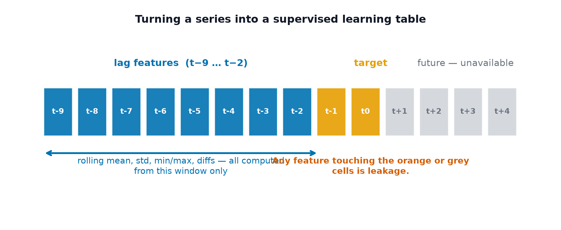
Reframe forecasting as supervised learning: each row is one timestamp, the features are lags and rolling statistics computed strictly from the past, and the target is a future value. Every feature must be computable at prediction time, or you have built a model that cannot run.
The feature families
| Family | Examples | Notes |
|---|---|---|
| Lags | y(t−1), y(t−7), y(t−364) | The workhorse. Include seasonal lags |
| Rolling statistics | mean/std/min/max over 7, 28, 91 days | Must be shifted — see below |
| Expanding statistics | cumulative mean, all-time max | Uses everything up to t−1 |
| Calendar | day of week, month, quarter, week of year | Cheap and often very strong |
| Event flags | holiday, promotion, outage | Frequently the largest single win |
| Cyclical encodings | sin(2πt/7), cos(2πt/7) | Keeps Sunday adjacent to Monday |
| Exogenous drivers | price, weather, marketing spend | Must be known or forecastable for the horizon |
df["y"].rolling(7).mean() at row t includes y(t) itself — the value you are trying to predict. You must shift:
df["roll7"] = df["y"].shift(1).rolling(7).mean()   # correct
df["roll7"] = df["y"].rolling(7).mean()            # LEAKS the current value
This single missing .shift(1) produces spectacular validation scores and a model that fails completely in production. Check every rolling feature for it.
Cyclical encoding
Encoding day-of-week as the integers 0–6 tells the model that Sunday (6) is six units from Monday (0), when it is actually one day away. Encoding it as a (sin, cos) pair on a circle fixes that:
df["dow_sin"] = np.sin(2 * np.pi * df["dow"] / 7)
df["dow_cos"] = np.cos(2 * np.pi * df["dow"] / 7)
Tree models care about this less than linear models and neural networks — a tree can carve out dow == 6 with a pair of splits — but it rarely hurts, and one-hot encoding is a perfectly good alternative for low-cardinality cycles.
Exogenous variables have a catch
A feature is only usable if it is available at prediction time for the whole horizon. Weather is a superb predictor of energy demand — but forecasting tomorrow's demand requires tomorrow's weather, which is itself a forecast carrying its own error.
Three cases, and they behave very differently:
| Kind | Example | Usable? |
|---|---|---|
| Known in advance | holidays, calendar, scheduled promotions | Yes, straightforwardly |
| Must be forecast | weather, competitor price | Only with its forecast error propagated |
| Only known afterwards | actual footfall, realised demand | Only as a lagged feature |
Direct, recursive, and multi-output
To forecast steps ahead you need one of three strategies:
| Strategy | How | Trade-off |
|---|---|---|
| Recursive | One 1-step model, fed its own predictions | Simple; errors compound over the horizon |
| Direct | A separate model per horizon | No compounding; h models to train and maintain |
| Multi-output | One model emitting all h at once | Captures horizon correlations; needs a supporting architecture |
Recursive is the default and is fine for short horizons. Direct wins as the horizon grows because a 14-step recursive forecast has fed its own errors back thirteen times. Note that direct models cannot use lag features shorter than their horizon — a 7-step-ahead model may not use y(t−1), because at prediction time that value does not yet exist.
Which model
| Model | When |
|---|---|
| Gradient boosting (LightGBM, XGBoost) | The default for tabular forecasting. Fast, handles many features, wins most competitions |
| Linear / ridge on lag features | Strong baseline, trivially interpretable |
| DeepAR, N-BEATS, TFT | Many related series, long horizons, need probabilistic output |
| Transformers (Informer, PatchTST) | Very long sequences; often beaten by simpler methods, so benchmark honestly |
A decision tree predicts by averaging training targets in a leaf, so its output can never leave the range it saw in training. On a series with a persistent upward trend, a gradient-boosted model will flatline at the highest value it has seen.
The fix is to remove the trend before modelling — fit on differences or on detrended residuals, then add the trend back — or to include time as a feature in a model that can extrapolate. This is the most common reason a boosted model loses to a naive drift forecast.
Where ML genuinely beats classical models
Not on a single short series — there, ARIMA and exponential smoothing usually win. ML pulls ahead when:
- there are many related series (thousands of products), so one model can learn shared patterns and borrow strength across them
- there are rich exogenous features — promotions, prices, holidays, weather
- relationships are non-linear or interacting (a promotion has different effects by weekday)
- the series are long enough to support a flexible model
The M5 competition is the reference point: LightGBM on engineered features dominated a hierarchy of 42,840 related retail series. The earlier M3 competition, on short independent series, was won by exponential smoothing.
Code: building the supervised table safely
import numpy as np
import pandas as pd


def make_supervised(df, target="y", lags=(1, 2, 3, 7, 14, 28),
                    windows=(7, 28), horizon=1):
    """Turn a time-indexed frame into a supervised table.

    Every feature is built from data strictly before the row's timestamp, so
    the result is safe to hand to any tabular model.
    """
    out = df.copy()

    for lag in lags:
        out[f"lag_{lag}"] = out[target].shift(lag)

    # .shift(1) BEFORE .rolling() is what excludes the current value.
    for w in windows:
        shifted = out[target].shift(1)
        out[f"roll_mean_{w}"] = shifted.rolling(w).mean()
        out[f"roll_std_{w}"] = shifted.rolling(w).std()
        out[f"roll_max_{w}"] = shifted.rolling(w).max()

    idx = out.index
    out["dow"] = idx.dayofweek
    out["month"] = idx.month
    out["dow_sin"] = np.sin(2 * np.pi * out["dow"] / 7)
    out["dow_cos"] = np.cos(2 * np.pi * out["dow"] / 7)

    out["target"] = out[target].shift(-horizon)      # what we predict
    return out.dropna()


def assert_no_leakage(frame, target="y"):
    """Any feature correlating ~perfectly with the target is a red flag."""
    suspects = []
    for col in frame.columns:
        if col in (target, "target"):
            continue
        c = frame[col].corr(frame["target"])
        if pd.notna(c) and abs(c) > 0.999:
            suspects.append((col, c))
    return suspects


if __name__ == "__main__":
    rng = np.random.default_rng(0)
    idx = pd.date_range("2022-01-01", periods=730, freq="D")
    trend = np.linspace(0, 30, 730)
    weekly = 8 * np.sin(2 * np.pi * np.arange(730) / 7)
    y = 100 + trend + weekly + rng.normal(0, 3, 730)
    df = pd.DataFrame({"y": y}, index=idx)

    table = make_supervised(df)
    print(f"{len(table)} rows, {table.shape[1]} columns")
    print("leakage suspects:", assert_no_leakage(table) or "none")

    # Chronological split — never shuffled.
    split = int(len(table) * 0.8)
    train, test = table.iloc[:split], table.iloc[split:]

    features = [c for c in table.columns if c not in ("y", "target")]
    X_tr = np.column_stack([np.ones(len(train)), train[features].to_numpy()])
    coefs, *_ = np.linalg.lstsq(X_tr, train["target"].to_numpy(), rcond=None)
    X_te = np.column_stack([np.ones(len(test)), test[features].to_numpy()])
    pred = X_te @ coefs

    actual = test["target"].to_numpy()
    naive = test["lag_1"].to_numpy()
    print(f"\nridge-free linear MAE : {np.mean(np.abs(actual - pred)):.2f}")
    print(f"naive (lag-1)    MAE : {np.mean(np.abs(actual - naive)):.2f}")
The comparison at the end is the point: a feature-engineered linear model should beat lag-1 persistence on a series with this much structure. If it does not, the features are not earning their complexity.
See also
- Validation and Backtesting — evaluating these models without leaking.
- Gradient Boosting — the model that wins most forecasting competitions.
- Data Preprocessing and Features — the general feature-engineering rules.