Validation and Backtesting

Every evaluation rule you learned for i.i.d. data is wrong here. Random k-fold cross-validation on a time series does not measure forecasting ability at all — it measures interpolation, and it reports a number far better than anything you will see in production.

Key idea

Validation must mimic deployment: train only on the past, predict only the future, and repeat that over several origins. A single train/test split gives one noisy estimate; rolling the origin forward gives a distribution.

Two backtesting schemes. The expanding window keeps all history and grows; the rolling window holds a fixed length and discards the distant past. In both, the evaluated block always sits immediately after the training block — never before it.

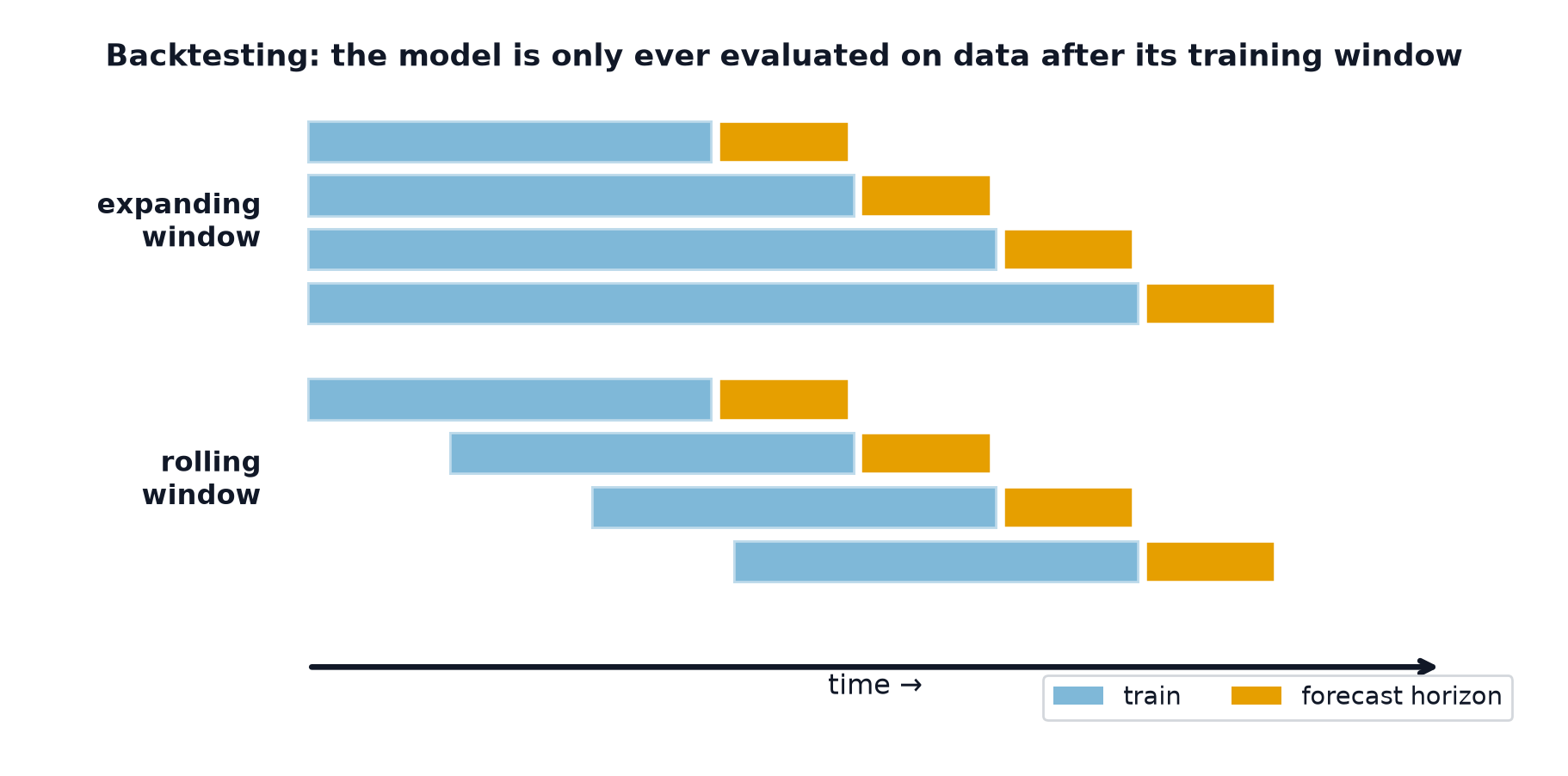
Expanding or rolling

	Expanding window	Rolling window
Training data	All history, growing	Fixed length, sliding
Assumes	The past stays relevant	Recent past is more relevant
Cost	Grows each fold	Constant
Use when	The process is stable	There are regime changes

Expanding is the usual default. Switch to rolling when you have evidence of a structural break, or when retraining cost matters — and note that the rolling window's length is a hyperparameter you should tune, not guess.

The gap you probably need

If your production model does not get labels immediately, validation must reproduce that delay. Suppose sales figures settle only after 7 days: at prediction time the model genuinely does not have the last week of data, so validation must not give it that either.

train ────────────────┃  gap  ┃ ─── test ───
                       (7 days)

Omitting the gap is a subtle, common leak. The model validates with information it will never have.

Metrics, and their failure modes

Metric	Formula	Breaks when
MAE	mean|y − ŷ|	Not scale-free; can't compare across series
RMSE	√mean(y − ŷ)²	Dominated by outliers
MAPE	mean|(y − ŷ)/y|	Undefined at y = 0; punishes over-forecasting more than under
sMAPE	symmetric variant	Still unstable near zero
MASE	MAE ÷ MAE of naive forecast	The safe default

MAPE is asymmetric and will bias your model

For an actual of 100, forecasting 50 gives 50 % error; forecasting 150 also gives 50 %. But forecasting 0 caps at 100 % while over-forecasting is unbounded. Optimising MAPE therefore systematically pushes forecasts down. On intermittent demand — where many actuals are zero — it is undefined outright.

Use MASE: it divides your error by the naive forecast's error on the training set, so a value below 1 means "better than naive" and values are comparable across series of any scale.

Forecast intervals

A point forecast without an interval is close to useless for decision-making — "we'll sell 500" and "we'll sell 500 ± 400" call for entirely different inventory choices.

Interval width grows with the horizon — roughly with √h for a random walk. A model reporting constant-width intervals across a long horizon is almost certainly miscalibrated.

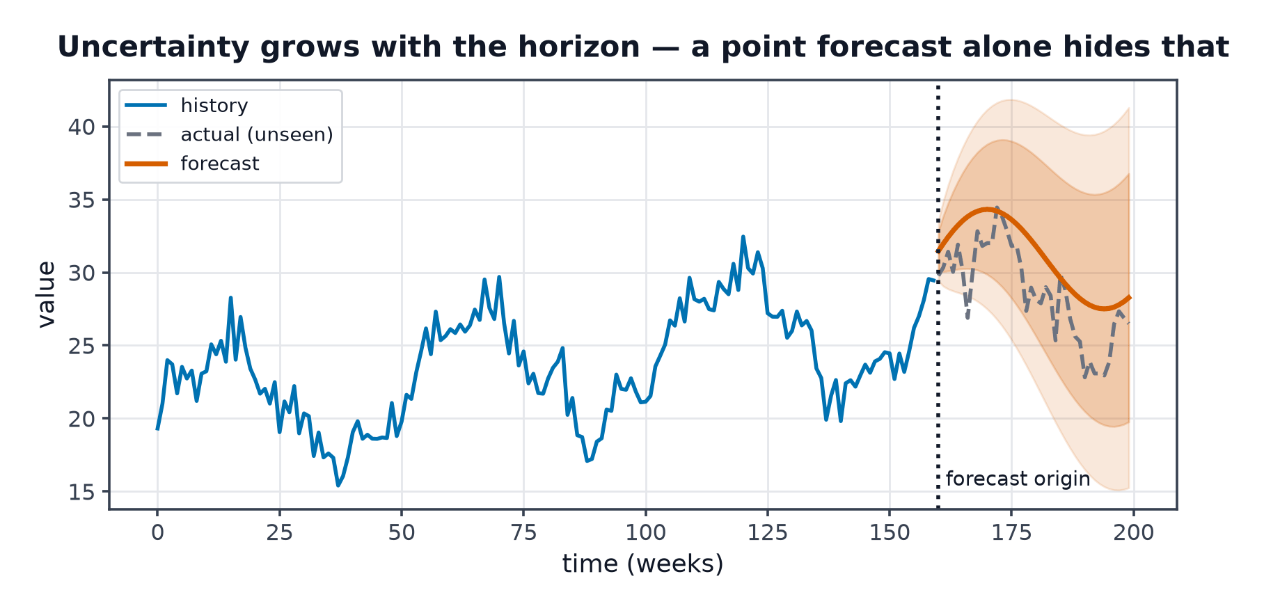
Evaluate intervals on coverage: over many forecasts, a 90 % interval should contain the actual about 90 % of the time. Measured coverage of 60 % means the model is overconfident, which is far more dangerous than a slightly worse point forecast. Pinball loss (quantile loss) scores the full predictive distribution and is what forecasting competitions increasingly use.

Pitfalls specific to time series

• Random k-fold. Trains on the future to predict the past. The headline error.
• Scaling before splitting. Fitting a scaler on the whole series leaks future mean and variance — same rule as in Data Preprocessing, and easier to get wrong here.
• Tuning on one split. Time series are noisy; a hyperparameter that wins on one origin often loses on the next. Tune across several origins and take the average.
• Ignoring the naive baseline. Reported often enough that it needs repeating.
• Aggregating errors across series of different scales. A MAE of 500 means something different for a product selling 10 units and one selling 100,000. Use MASE, or aggregate weighted.
• Evaluating one horizon when you deploy another. Errors at h = 1 say very little about h = 28.

Code: rolling-origin backtesting with MASE

backtest.py

import numpy as np


def mase(actual, predicted, train, season=1):
    """Mean absolute scaled error.

    Denominator is the in-sample MAE of the seasonal naive forecast, so
    MASE < 1 means "better than naive" and the value is scale-free.
    """
    actual, predicted, train = map(np.asarray, (actual, predicted, train))
    naive_error = np.mean(np.abs(train[season:] - train[:-season]))
    if naive_error == 0:
        return np.nan
    return np.mean(np.abs(actual - predicted)) / naive_error


def rolling_origin_backtest(series, forecast_fn, horizon=7, n_splits=5,
                            gap=0, min_train=60, expanding=True):
    """Evaluate `forecast_fn(history, horizon)` over several forecast origins.

    Returns one MASE per split. Reporting the spread matters as much as the
    mean: a model that is excellent on three origins and terrible on two is
    not a model you can deploy.
    """
    series = np.asarray(series, dtype=float)
    total = len(series)
    step = (total - min_train - gap - horizon) // max(n_splits - 1, 1)

    scores = []
    for i in range(n_splits):
        train_end = min_train + i * step
        test_start = train_end + gap
        test_end = test_start + horizon
        if test_end > total:
            break

        history = series[:train_end] if expanding else series[train_end - min_train:train_end]
        actual = series[test_start:test_end]
        scores.append(mase(actual, forecast_fn(history, horizon), history))
    return np.array(scores)


if __name__ == "__main__":
    rng = np.random.default_rng(7)
    t = np.arange(365)
    y = 200 + 0.15 * t + 25 * np.sin(2 * np.pi * t / 7) + rng.normal(0, 6, 365)

    def naive(history, h):
        return np.repeat(history[-1], h)

    def seasonal_naive(history, h):
        return np.array([history[-7 + (i % 7)] for i in range(h)])

    def drift(history, h):
        slope = (history[-1] - history[0]) / (len(history) - 1)
        return history[-1] + slope * np.arange(1, h + 1)

    for name, fn in [("naive", naive), ("seasonal naive", seasonal_naive), ("drift", drift)]:
        s = rolling_origin_backtest(y, fn, horizon=14, n_splits=6)
        print(f"{name:>16}: MASE {s.mean():.3f} ± {s.std():.3f}   per-split {np.round(s, 2)}")

    print("\nMASE < 1 beats the in-sample naive benchmark;")
    print("the spread across origins tells you whether that result is stable.")

Reporting the standard deviation across origins is not decoration. A model averaging MASE 0.8 with a spread of 0.5 is a different proposition from one averaging 0.85 with a spread of 0.05, and the mean alone cannot distinguish them.

See also

• Machine Learning for Forecasting — the models this evaluates.
• Train/Validation/Test Splits — the general case.
• Offline Evaluation — the same discipline in production terms.